Lecture 9

Simple Linear Regression Inference and Diagnostics

Linear regression itself does not require statistics to be done and one needs few assumptions for the ability to estimate a regression model. Statistics steps in when one wants to study the properties of a regression model. Using statistics, we can make statements about what the value of the population parameters are, decide between competing models, express uncertainty in mean values and predictions, and more. We will see techniques as well for assessing the quality of a model.

For reference, here’s the regression model we are considering:

\[y_i = \beta_0 + \beta_1 x_{1i} + \cdots + \beta_k x_{ki} + \epsilon_i.\]

Residual Properties

Linear models fitted via lm() can be plotted using plot(). The result is a sequence of four plots useful for assessing the quality of a linear model fit. This is in addition to a basic plot visualizing the linear model with the data.

(fit <- lm(Sepal.Length ~ Sepal.Width, data = iris,
           subset = Species == "setosa"))

## 
## Call:
## lm(formula = Sepal.Length ~ Sepal.Width, data = iris, subset = Species == 
##     "setosa")
## 
## Coefficients:
## (Intercept)  Sepal.Width  
##      2.6390       0.6905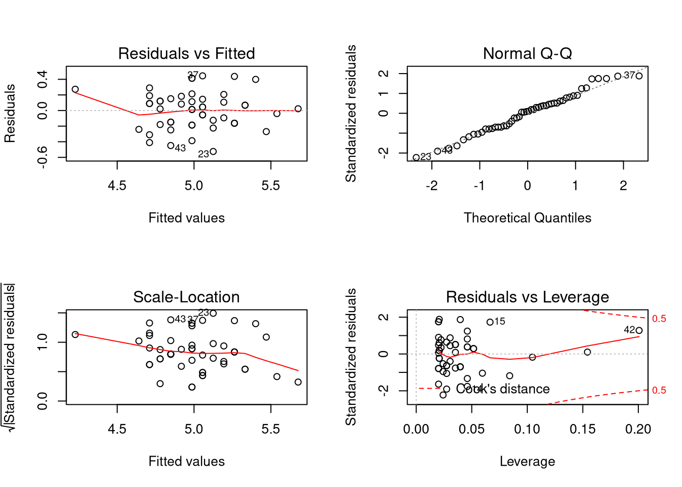

old_par <- par()
par(mfrow = c(2, 2))
plot(fit)

par(old_par)

## Warning in par(old_par): graphical parameter "cin" cannot be set

## Warning in par(old_par): graphical parameter "cra" cannot be set

## Warning in par(old_par): graphical parameter "csi" cannot be set

## Warning in par(old_par): graphical parameter "cxy" cannot be set

## Warning in par(old_par): graphical parameter "din" cannot be set

## Warning in par(old_par): graphical parameter "page" cannot be set

The meaning of these plots, from left to right and top to bottom:

We plot the estimated residuals of the model against the predicted value of the observations in the data set, according to the model. What we want to see is a “cloudy” shape, with no particularly strong patterns. Patterns could indicate an inappropriate model form; a simple linear model may not be appropriate and perhaps a different functional form is needed. We would also want to see constant “spread” in the data. If it seems that data is more spread out for some predicted values than others, this could indicate a phenomenon known as heteroskedasticity in the data (where the variance of the residuals depend on the data). We want the red line to be roughly straight. My own opinion is that for the plot above, the line is straight enough and there’s no strong evidence of heteroskedasticity (that is, the data is homoskedastic).
We create a Q-Q plot for the residuals of the data to see if they appear to be Normally distributed. Statistical procedures often assume Normally distributed residuals. We may be able to proceed without Normally distributed residuals, but some common procedures (such as prediction intervals) may fail.
This is a scale-location plot, which compares predicted values to the square root of the absolute value of the residuals. This plot is useful for identifying heteroskedasticity in the model. We want a “cloudy” shape with a roughly straight and flat red line. That appears to be the case here.
Least-squares regression ties intimately to the concept of mean and standard deviation, and as you should know from previous studies, means and standard deviations are affected by strong outliers. The notion of “outlier” is murkier in the regression context, yet still we care about “influential points”. The final plot compares the residuals to their leverage. In short, what we are looking for are points that fall outside a quantity known as Cook’s distance, which manifests as a point in one of the corners on the right-hand side of the plot outside of the Cook’s distance bands. Such points seem to have a strong influence on the resulting regression line and removing them could result in a regression line quite different from before. In this case, while one observation gets close to the Cook’s distance band, it doesn’t cross, and thus it doesn’t appear that there are strong outliers “biasing” our regression estimates.

(The above plots actually work with standardized residuals, or the residuals scaled to have variance 1.)

Compare the above model to a model estimated for home runs against at bats in the batting (UsingR) data set.

library(UsingR)

## Loading required package: HistData

## Loading required package: Hmisc

## Loading required package: lattice

## Loading required package: survival

## Loading required package: Formula

## Loading required package: ggplot2

## 
## Attaching package: 'Hmisc'

## The following objects are masked from 'package:base':
## 
##     format.pval, units

## 
## Attaching package: 'UsingR'

## The following object is masked from 'package:survival':
## 
##     cancer

(fit2 <- lm(HR ~ AB, data = batting))

## 
## Call:
## lm(formula = HR ~ AB, data = batting)
## 
## Coefficients:
## (Intercept)           AB  
##    -2.94675      0.04067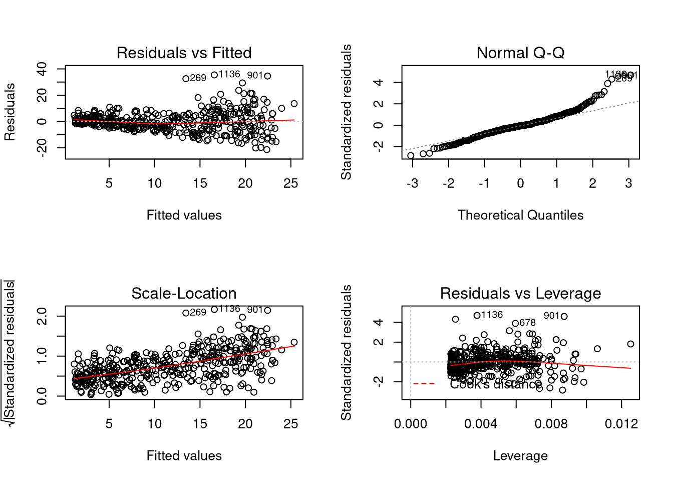

old_par <- par()
par(mfrow = c(2, 2))
plot(fit2)

par(old_par)

## Warning in par(old_par): graphical parameter "cin" cannot be set

## Warning in par(old_par): graphical parameter "cra" cannot be set

## Warning in par(old_par): graphical parameter "csi" cannot be set

## Warning in par(old_par): graphical parameter "cxy" cannot be set

## Warning in par(old_par): graphical parameter "din" cannot be set

## Warning in par(old_par): graphical parameter "page" cannot be set

Model Inference

Given an lm() fit called fit, we can see tables containing statistical results for our models using stargazer(fit) or summary(fit).

(inf <- summary(fit))  # Saving summary results; could be useful

## 
## Call:
## lm(formula = Sepal.Length ~ Sepal.Width, data = iris, subset = Species == 
##     "setosa")
## 
## Residuals:
##      Min       1Q   Median       3Q      Max 
## -0.52476 -0.16286  0.02166  0.13833  0.44428 
## 
## Coefficients:
##             Estimate Std. Error t value Pr(>|t|)    
## (Intercept)   2.6390     0.3100   8.513 3.74e-11 ***
## Sepal.Width   0.6905     0.0899   7.681 6.71e-10 ***
## ---
## Signif. codes:  0 '***' 0.001 '**' 0.01 '*' 0.05 '.' 0.1 ' ' 1
## 
## Residual standard error: 0.2385 on 48 degrees of freedom
## Multiple R-squared:  0.5514, Adjusted R-squared:  0.542 
## F-statistic: 58.99 on 1 and 48 DF,  p-value: 6.71e-10

str(inf)

## List of 11
##  $ call         : language lm(formula = Sepal.Length ~ Sepal.Width, data = iris, subset = Species ==      "setosa")
##  $ terms        :Classes 'terms', 'formula'  language Sepal.Length ~ Sepal.Width
##   .. ..- attr(*, "variables")= language list(Sepal.Length, Sepal.Width)
##   .. ..- attr(*, "factors")= int [1:2, 1] 0 1
##   .. .. ..- attr(*, "dimnames")=List of 2
##   .. .. .. ..$ : chr [1:2] "Sepal.Length" "Sepal.Width"
##   .. .. .. ..$ : chr "Sepal.Width"
##   .. ..- attr(*, "term.labels")= chr "Sepal.Width"
##   .. ..- attr(*, "order")= int 1
##   .. ..- attr(*, "intercept")= int 1
##   .. ..- attr(*, "response")= int 1
##   .. ..- attr(*, ".Environment")=<environment: R_GlobalEnv> 
##   .. ..- attr(*, "predvars")= language list(Sepal.Length, Sepal.Width)
##   .. ..- attr(*, "dataClasses")= Named chr [1:2] "numeric" "numeric"
##   .. .. ..- attr(*, "names")= chr [1:2] "Sepal.Length" "Sepal.Width"
##  $ residuals    : Named num [1:50] 0.0443 0.1895 -0.1486 -0.1795 -0.1248 ...
##   ..- attr(*, "names")= chr [1:50] "1" "2" "3" "4" ...
##  $ coefficients : num [1:2, 1:4] 2.639 0.6905 0.31 0.0899 8.5125 ...
##   ..- attr(*, "dimnames")=List of 2
##   .. ..$ : chr [1:2] "(Intercept)" "Sepal.Width"
##   .. ..$ : chr [1:4] "Estimate" "Std. Error" "t value" "Pr(>|t|)"
##  $ aliased      : Named logi [1:2] FALSE FALSE
##   ..- attr(*, "names")= chr [1:2] "(Intercept)" "Sepal.Width"
##  $ sigma        : num 0.239
##  $ df           : int [1:3] 2 48 2
##  $ r.squared    : num 0.551
##  $ adj.r.squared: num 0.542
##  $ fstatistic   : Named num [1:3] 59 1 48
##   ..- attr(*, "names")= chr [1:3] "value" "numdf" "dendf"
##  $ cov.unscaled : num [1:2, 1:2] 1.689 -0.487 -0.487 0.142
##   ..- attr(*, "dimnames")=List of 2
##   .. ..$ : chr [1:2] "(Intercept)" "Sepal.Width"
##   .. ..$ : chr [1:2] "(Intercept)" "Sepal.Width"
##  - attr(*, "class")= chr "summary.lm"

library(stargazer)
stargazer(fit, type = "text")

## 
## ===============================================
##                         Dependent variable:    
##                     ---------------------------
##                            Sepal.Length        
## -----------------------------------------------
## Sepal.Width                  0.690***          
##                               (0.090)          
##                                                
## Constant                     2.639***          
##                               (0.310)          
##                                                
## -----------------------------------------------
## Observations                    50             
## R2                             0.551           
## Adjusted R2                    0.542           
## Residual Std. Error       0.239 (df = 48)      
## F Statistic           58.994*** (df = 1; 48)   
## ===============================================
## Note:               *p<0.1; **p<0.05; ***p<0.01

Let’s explain these tables.

Coefficient Standard Errors

The estimated regression coefficients are statistics estimated from a sample, so like other statistics you’ve seen (sample mean or sample proportion), they have a standard error. The estimated standard error is given below:

vcov(fit)

##             (Intercept)  Sepal.Width
## (Intercept)  0.09610887 -0.027704441
## Sepal.Width -0.02770444  0.008081809

Actually I lied. When discussing regression models the notion of “standard error” still exists but needs to change. See, we’re not estimating just one statistic, but two: a slope and an intercept term. As a result, we need to account not just for how the two statistics themselves vary but also how the statistics vary jointly. That is, we need to account for correlation in the sample estimates.

The above matrix produced by the function vcov() is a covariance matrix, where the entries on the diagonal of the matrix are variances of random variables and the off-diagonal entries are the covariances between respective random variables. (Since the covariance is a symmetric function, all covariance matrices are symmetric. Additionally, since variances are non-negative, the diagonal of a covariance matrix is non-negative. In fact there are many properties of covariance matrices that are ultimately linear algebra discussions we won’t have here.) in this case, the diagonal of the matrix produced by vcov() contains squared standard errors of the coefficients while the off-diagonal entries are the covariances between those parameter estimates. If we want correlations we can call cov2cor() on the covariance matrix.

cov2cor(vcov(fit))

##             (Intercept) Sepal.Width
## (Intercept)   1.0000000  -0.9940617
## Sepal.Width  -0.9940617   1.0000000

For this correlation matrix, the diagonal entries are all 1 since random variables are perfectly correlated with themselves. The interesting part is the off-diagonal entries; here we see extremely strong negative correlations. Our interpretation of this is that the intercept and the slope term of the regression line vary in opposite directions; if the slope term is too small, the intercept term probably is too large.

That said, if we want the standard errors of the coefficients without considering their covariation, we can extract the diagonal of the covariance matrix using the function diag() (which is also the function used for creating diagonal matrices from vectors in R). Then we can take the square root of the result to get the standard errors of the coefficients.

coef_stderr <- function(...) {
  sqrt(diag(vcov(...)))
}

coef_stderr(fit)

## (Intercept) Sepal.Width 
##  0.31001431  0.08989888

Compare the above to the output of summary(fit).

\(t\)-Tests

Consider the following matrix:

inf$coefficients

##              Estimate Std. Error  t value     Pr(>|t|)
## (Intercept) 2.6390012 0.31001431 8.512514 3.742438e-11
## Sepal.Width 0.6904897 0.08989888 7.680738 6.709843e-10

Notice the last two columns. We can perform hypothesis testing to determine the value of the population coefficients corresponding with our estimates. That is, we can decide between:

\[H_0: \beta_j = \beta_{j0}\]

and

\[H_A: \begin{cases} \beta_{j} < \beta_{j0} \\ \beta_{j} \neq \beta_{j0} \\ \beta_{j} > \beta_{j0} \end{cases}\]

Assume that the standard errors \(\epsilon_i\) in the regression model are i.i.d. and Normally distributed with mean zero. Then we can decide between \(H_0\) and \(H_A\) by using the \(t\)-statistic:

\[t = \frac{\hat{\beta}_j - \beta_{k0}}{SE(\hat{\beta}_j)}\]

where \(SE(\hat{\beta}_j)\) is the standard error of the statistic \(\hat{\beta}_j\). Under the null hypothesis, the \(t\)-statistic follows a \(t(n - k - 1)\) distribution; notice that the degrees of freedom of the statistic is \(n - k - 1\), not \(n - 1\). Generally in statistics, the degrees of freedom are \(n\) minus the number of parameters being estimated. In the simple mean testing context, one parameter was estimated: the mean, \(\mu\). In fact, we can view hypothesis testing in that context as inference for the mean model:

\[y_i = \mu + \epsilon_i.\]

In linear regression, there are \(k + 1\) parameters being estimated: the \(k\) slope terms plus the intercept term. (If suppressing the constant, there would be \(k\) parameters estimated, so the degrees of freedom would be \(n - k\).)

Otherwise hypothesis tests regarding the value of regression coefficients are exactly like the \(t\)-tests you’ve seen before. summary.lm() reports the results for hypothesis tests checking whether the coefficients are zero or not. (That is, the tests are two-sided and \(\beta_{j0} = 0\).) This is the default hypothesis test in linear regression models since it translates to whether an explanatory variables has a linear effect on a response variable or not. If not, it may be inappropriate to include the variable in the model.

The regression table returned by stargazer() more closely resembles regression tables commonly seen in papers and books, with standard errors reported below coefficient estimates and stars appearing beside the coefficients. More stars appear for increasingly small \(p\)-values, and the cutoffs for the number of stars shown should be listed nearby. (Notice that summary.lm() also uses stars but at a different scale than that given by stargazer().)

Of course, we can do our own hypothesis tests for what values the coefficients should be. First let’s compute \(t\)-statistics:

coef_tstat <- function(fit, beta0 = 0) {
  se <- coef_stderr(fit)
  beta <- coef(fit)
  (beta - beta0) / se
}

coef_tstat(fit)

## (Intercept) Sepal.Width 
##    8.512514    7.680738

coef_tstat(fit, beta0 = c(2, 1))

## (Intercept) Sepal.Width 
##    2.061199   -3.442871

Then compute degrees of freedom.

deg_free <- function(fit) {
  n <- length(resid(fit))
  k <- length(coef(fit))
  n - k
}

deg_free(fit)

## [1] 48

Then we can test a one-side alternative hypothesis (in thise case, \(H_A: \beta_0 > 2\)) like so:

pt(coef_tstat(fit, beta0 = 2)[1], df = deg_free(fit), lower.tail = FALSE)

## (Intercept) 
##  0.02236164

Confidence Intervals

In mean models we compute confidence intervals for the mean. Naturally we would like to compute confidence intervals for the population model coefficients as well. However, since we’re estimating multiple parameters, the conversation isn’t quite the same.

On the one hand we can consider an interval for each \(\beta_{j}\) without concerning ourselves with the values of the other coefficients. If we wanted a confidence interval for just \(\beta_j\), we could compute one using

\[\hat{\beta}_j \pm t^* SE(\hat{\beta}_j)\]

with \(t^*\) be the corresponding critical value from a \(t\) distribution with \(n - k - 1\) degrees of freedom.

The code below obtains confidence intervals for each of the parameters in the model in this way.

coef_conf_int <- function(fit, conf.level = 0.95) {
  beta <- coef(fit)
  se <- coef_stderr(fit)
  nu <- deg_free(fit)
  tstar <- qt((1 - conf.level) / 2, df = nu, lower.tail = FALSE)
  moe <- se * tstar
  cbind(lower = beta - moe, upper = beta + moe)
}

coef_conf_int(fit)

##                 lower     upper
## (Intercept) 2.0156757 3.2623268
## Sepal.Width 0.5097359 0.8712435

However, these are marginal confidence intervals that are valid when considering the model parameters separately. The join confidence interval (where we hope that both \(\beta_0\) and \(\beta_1\) fall into the region) is quite different. For starters, a confidence “interval” doesn’t make sense when talking about something that is essentially two-dimensional: the vector \((\beta_0, \beta_1)^\top\). Instead we need to talk about a confidence region, a set (this time in a two-dimensional plane) that hopefully contains the values of the population parameters. (In general, these sets are subsets of \(k + 1\) dimensional space; remember that \(k\) is the number of parameters in the model excluding the intercept and residual standard deviation.) If we were to use just the marginal confidence intervals found above, the resulting region would be a square/cube/hypercube, but the probability the resulting region would capture the parameter values would not be the confidence level. Thus such a region is inappropriate.

Statisticians often consider a confidence ellipse (in high dimensions this would be a hyperellipse, but we’ll still call it an ellipse). A confidence ellipse accounts for the correlation in the sample estimates, and any point in the ellipse represents a plausible combination of values for the true parameter coefficients.

The ellipse package allows for visualizing confidence ellipses. Below I show how it can be used for visualizing a confidence ellipse.

library(ellipse)

## 
## Attaching package: 'ellipse'

## The following object is masked from 'package:graphics':
## 
##     pairs

plot_conf_ellipse <- function(..., col = 1, add = FALSE) {
  if (add) {
    pfunc = lines
  } else {
    pfunc = plot
  }
  pfunc(ellipse(...), type = "l", col = col)
}

plot_conf_ellipse(fit)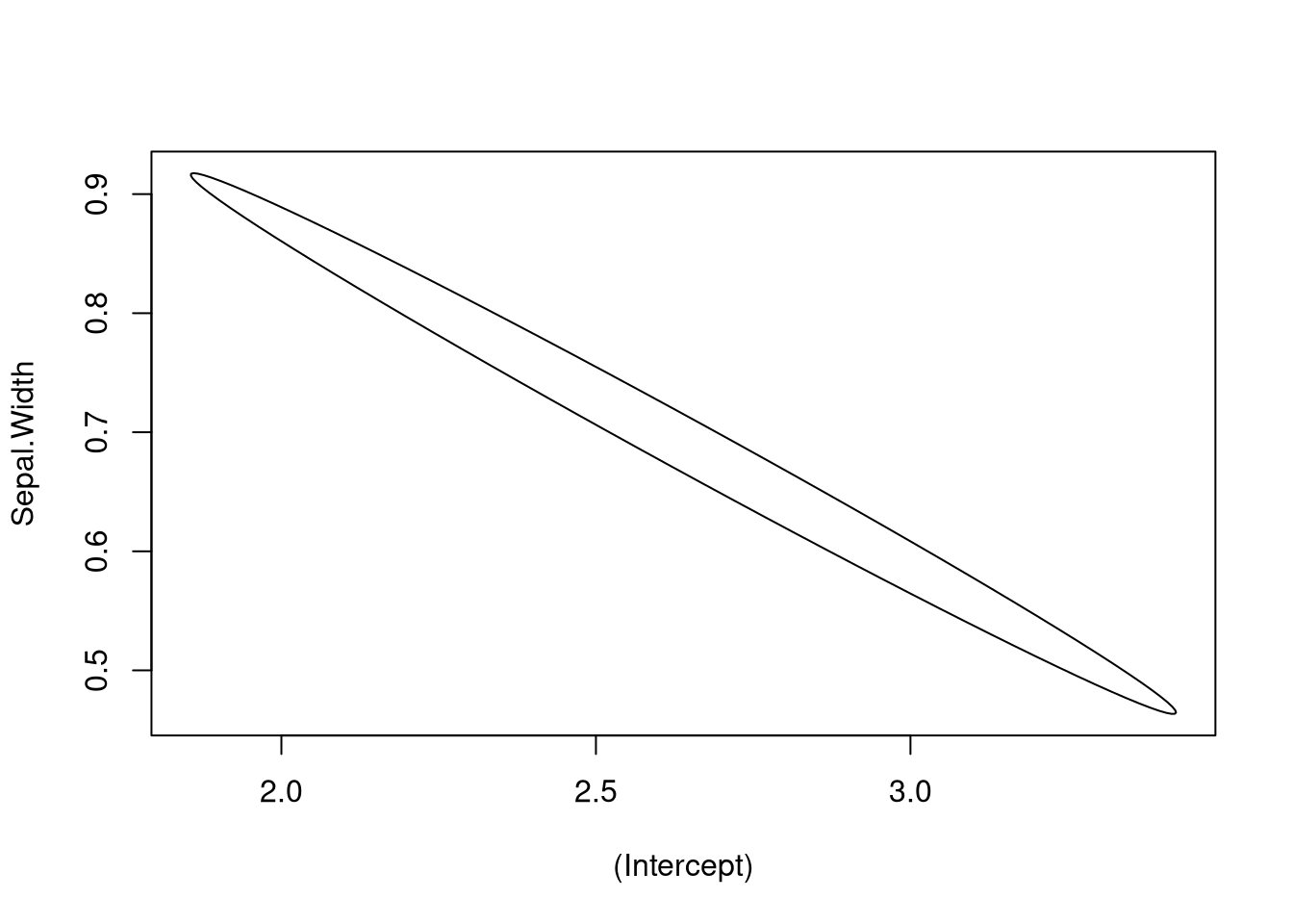

plot_conf_ellipse(fit, level = 0.99)
plot_conf_ellipse(fit, level = 0.95, add = TRUE, col = 2)
plot_conf_ellipse(fit, level = 0.90, add = TRUE, col = 3)
points(coef(fit)[1], coef(fit)[2], pch = 20)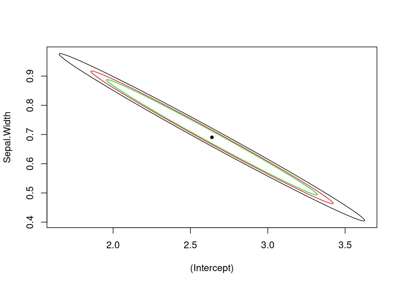

Our takeaway from the above plots is that the coefficient estimates for the intercept and slope terms are highly correlated, and if the slope is too small, the intercept is likely to be too large.

\(R^2\)

The \(R^2\) value, also known as the coefficient of determination, is a measure of how well the regression line fits the data. If \(SSE = \sum_{i=1}^n (y_i - \bar{y})^2\) and \(SSR = \sum_{i = 1}^n (\hat{y}_i - \bar{y})^2\), then

\[R^2 = 1 - \frac{SSR}{SSE}.\]

The \(R^2\) value can be interpreted as the percentage of variation in the response variable that can be explained by variation in the explanatory variable. In fact, it turns out that in this simple linear regression context, \(R^2 = r^2\), where \(r\) is the correlation coefficient. In this way one can generalize the notion of correlation to more than one variable (the other way is the covariance matrix).

We can extract \(R^2\) from the summary of a linear model like so:

inf$r.squared

## [1] 0.5513756

Despite the interpretation presented above, don’t get too excited about interpreting \(R^2\). Just because \(R^2\) is high doesn’t mean there is a causal relationship between the variables; it just means there’s an association between them.

Adjusted \(R^2\) is interpreted like \(R^2\) but accounts for the number of parameters in the model. It turns out that \(R^2\) cannot decrease as one adds more variables, so one could increase \(R^2\) by adding irrelevant variables to the model. (The resulting model would be considered overfitted, where errors in the estimated model are small but the model behaves poorly out of sample.) Adjusted \(R^2\) is a penalized version of \(R^2\) and equals \(\bar{R}^2 = 1 - (1 - R^2) \frac{n - 1}{n - k - 1}\).

We can extract adjusted \(R^2\) using:

inf$adj.r.squared

## [1] 0.5420292

In the case of simple linear regression the distinction between the two metrics matters little, but for more complex models we almost always consider adjusted \(R^2\) rather than \(R^2\).

\(F\)-Test

The \(F\) test can be used to determine if additional coefficients in a regression model in some sense “add value” to the model; more specifically, it checks if all additional coefficients are zero or not. Here we would be using the \(F\)-test to decide if the simple linear regression model is better than the mean model.

The \(F\) statistic is used for inference and can be extracted from the summary of a linear model like so:

inf$fstatistic

##    value    numdf    dendf 
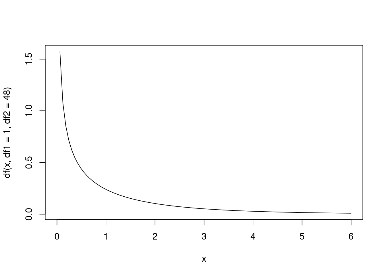
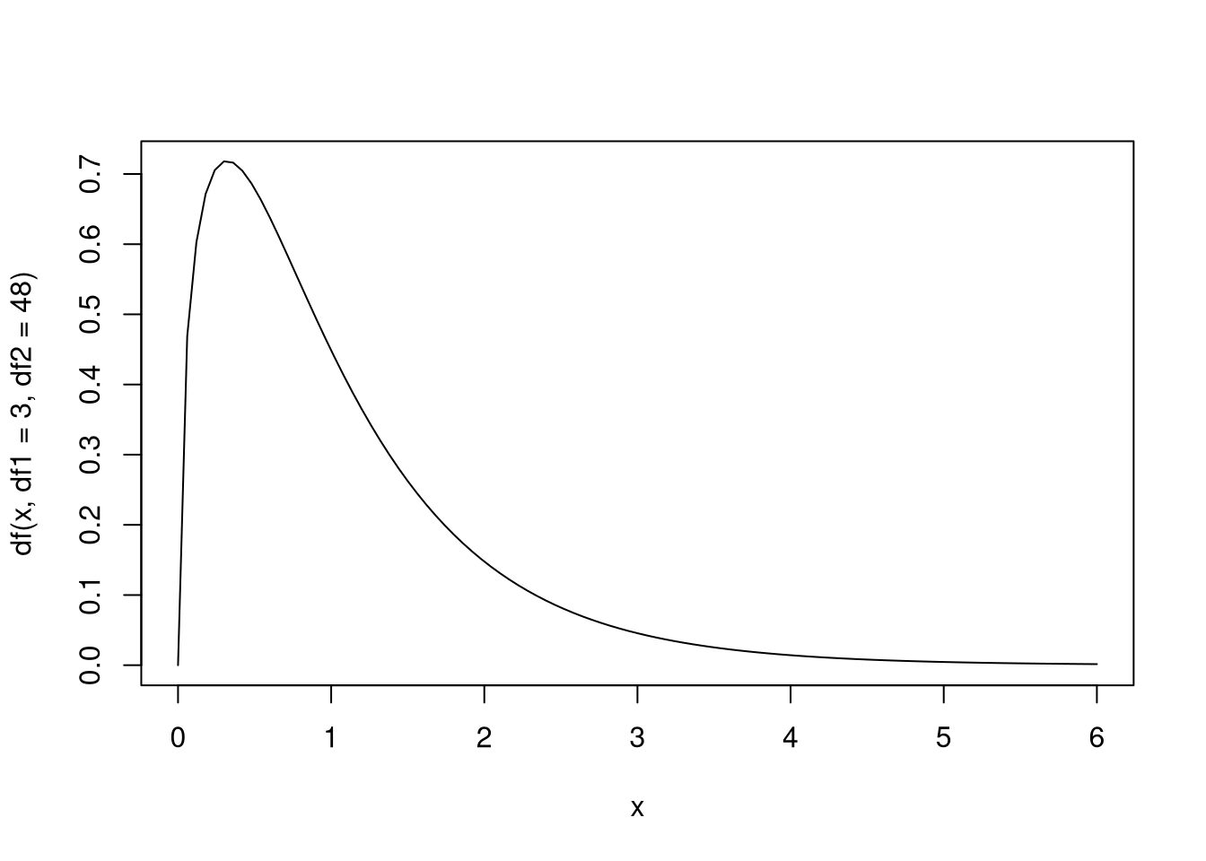
## 58.99373  1.00000 48.00000

Inference with the \(F\) statistic is done using the \(f\) distribution, which depends on two parameters: the numerator degrees of freedom and the denominator degrees of freedom. If \(X\) is an \(f\)-distributed random variable, we say \(X \sim f(\nu_{\text{num}}, \nu_{\text{den}})\), where \(\nu_{\text{num}}\) and \(\nu_{\text{den}}\) are the numerator and denominator degrees of freedom, respectively. In this case, if we denote the observed \(f\) statistic with \(\hat{f}\), the \(p\)-value is computed via \(P(X > \hat{f})\).

Here is a visualization of the \(F\) distribution.

curve(df(x, df1 = 1, df2 = 48), from = 0, to = 6)

curve(df(x, df1 = 3, df2 = 48), from = 0, to = 6)

Below is a function that computes the \(p\)-value for the \(F\) test:

ftest_pval <- function(fit) {
  f <- summary(fit)$fstatistic
  pf(f[["value"]], df1 = f[["numdf"]], df2 = f[["dendf"]], lower.tail = FALSE)
}

ftest_pval(fit)

## [1] 6.709843e-10

The \(p\)-value for this model is very small, suggesting that the explanatory variable belongs in our linear model for the response variable. (Well, whether it “belongs” is a strong statement; there could be a better model not including this variable.) For now the \(F\)-test doesn’t seem to offer any advantage over tests for just the regression coefficients, but one should note that the two are not the same and one is not a substitute for the other. Particularly, for models with multiple explanatory variables, just because none of the explanatory variables’ regression coefficients are statistically different from zero doesn’t mean that the mean model is better than the regression model. On the flip side, a single statistically significant coefficient in a large linear model could be a false positive; the result of the \(F\) test would warn of this possibility. The \(F\) test again represents an overall test for statistical significance while the \(t\)-tests would be individual tests helping decide which coefficients are not zero.

The \(f\)-test can also be used to decide between a regression model and another model with more explanatory variables. We will revisit such a test later.

Point-Wise Inference

Our inference procedures so far have focused on the properties of the model, but we can also have discussions about the value of the model at particular points, for select values of the explanatory variables. If \(Y\) represents the response variable understood as a random variable, we are studying the behavior of \(Y \mid| X = x\), where \(X\) is the explanatory variable viewed as a random variable. We would like to address two particular questions:

What is the expected value of \(Y\) given \(X = x\)? That is, what is the conditional mean of \(Y\) when \(X = x\)? We will answer this with a point-wise confidence interval.
If we know \(X = x\), what are plausible values of \(Y\)? That is, we would like to predict the value of \(Y\) given \(X = x\); this is a point-wise prediction interval.

Again we will assume that the residuals are Normally distributed. If the sample size is large this won’t matter for point-wise confidence intervals, but this assumption matters for prediction intervals at any sample size.

The function predict() when called on an lm-class object gives estimated conditional means for regression models, but it also does more. It can also give confidence and prediction intervals. Let’s write a function returning a closure giving an easy interface to predict() for a given data set.

predict_func <- function(fit) {
  response <- names(fit$model)[[1]]
  explanatory <- names(fit$model)[[2]]
  function(x, ...) {
    dat <- data.frame(x)
    names(dat) <- explanatory
    predict(fit, dat, ...)
  }
}

Let’s demonstrate the closure on the iris model.

sepal_line <- predict_func(fit)
sepal_line(2:4)

##        1        2        3 
## 4.019981 4.710470 5.400960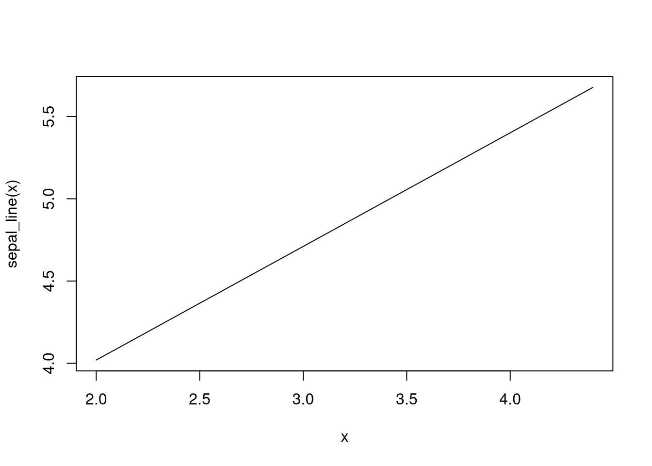

with(iris, {
  curve(sepal_line, from = min(Sepal.Width), to = max(Sepal.Width))
})

Now note that the arguments being passed to sepal_line() other than the first argument x are actually arguments for predict(). We just made a nicer interface for predict(). Anyway, predict() is able to compute both point-wise confidence and prediction intervals. We do so by setting the interval argument to either "confidence" or "prediction", depending on our desires. By default these are 95% intervals, but we can change the level by setting the level argument.

sepal_line(2:4, interval = "confidence", level = 0.99)  # Point-wise CIs

##        fit      lwr      upr
## 1 4.019981 3.663961 4.376001
## 2 4.710470 4.573218 4.847722
## 3 5.400960 5.236004 5.565916

sepal_line(2:4, interval = "prediction", level = 0.99)  # Point-wise PIs

##        fit      lwr      upr
## 1 4.019981 3.287780 4.752182
## 2 4.710470 4.056096 5.364845
## 3 5.400960 4.740219 6.061701

Note that what’s returned is a matrix with three columns; the first is a column with the value of the regression line at that point, the second column the lower bound of the interval, the third the upper bound.

We would like to visualize these intervals. The function below will plot these intervals along with the original data.

plot_fit <- function(fit, interval = "confidence", level = 0.95, len = 1000,
                     ...) {
  fit_func <- predict_func(fit)
  x_range <- c(min(fit$model[[2]]), max(fit$model[[2]]))
  x_vals <- seq(from = x_range[[1]] * 0.9, to = x_range[[2]] * 1.1,
                length = len)
  interval_mat <- fit_func(x_vals, interval = interval, level = level)
  y_range <- c(min(c(interval_mat[, 2], fit$model[[1]])),
               max(c(interval_mat[, 3], fit$model[[1]])))
  plot(fit$model[2:1], xlim = x_range, ylim = y_range, ...)
  abline(fit)
  lines(x_vals, interval_mat[, 2], col = "red")
  lines(x_vals, interval_mat[, 3], col = "red")
}

plot_fit(fit, main = "Conditional CIs", pch = 20)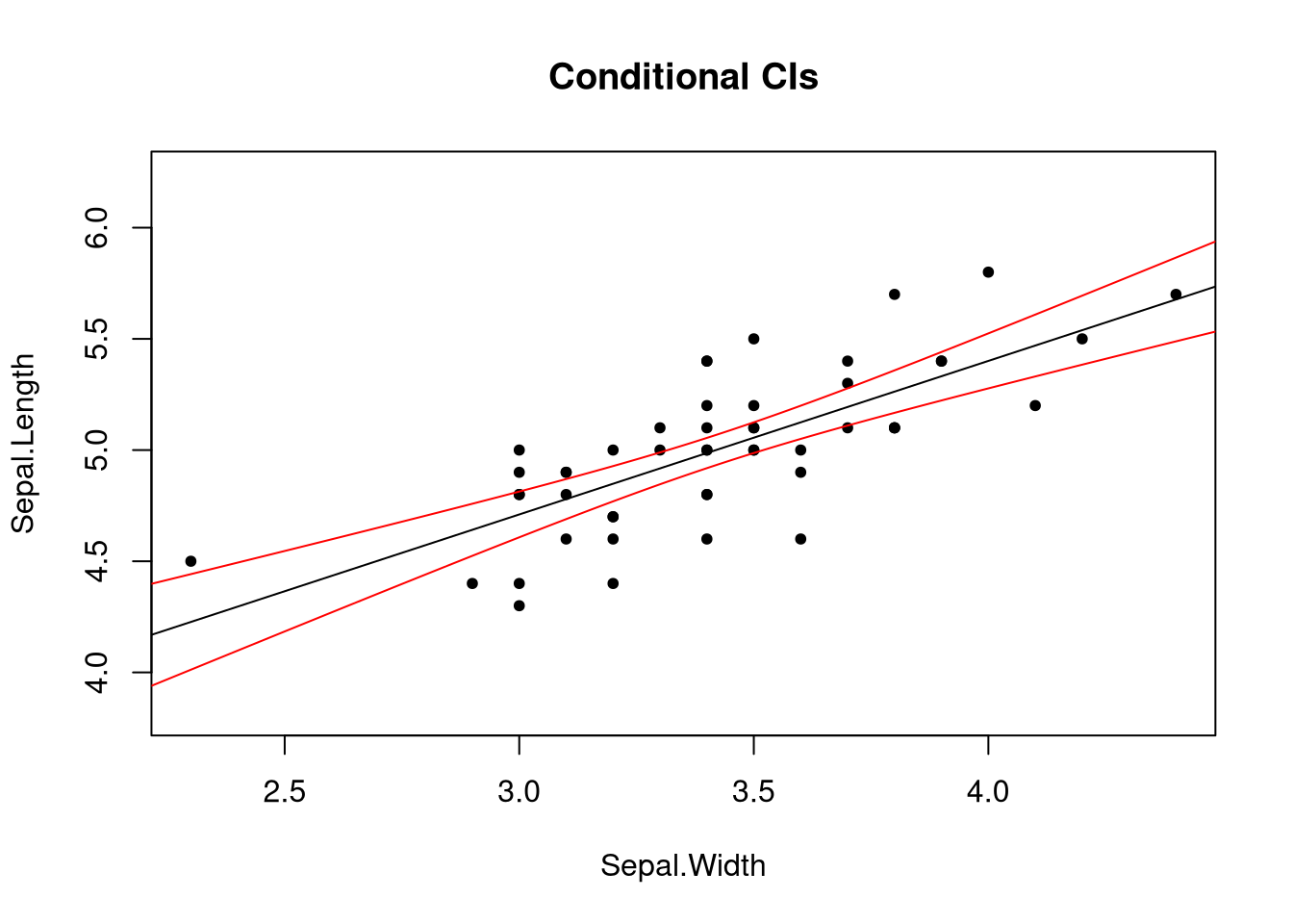

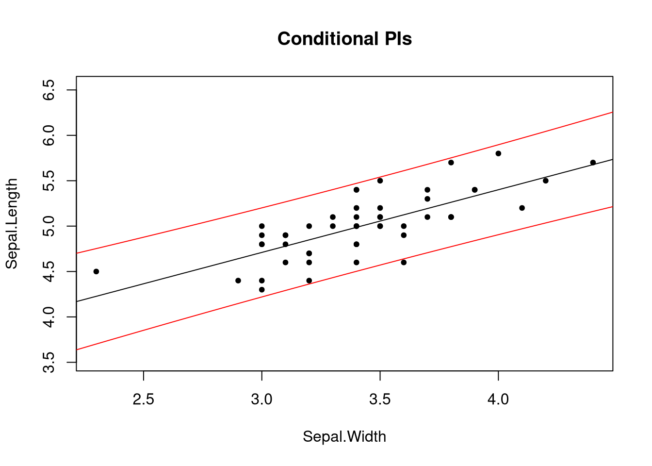
plot_fit(fit, main = "Conditional PIs", pch = 20, interval = "prediction")

Notice two things: one, the intervals are curved. The uncertainty of our estimates increases as we approach the ends of the range of the explanatory variable. Two, prediction intervals are wider than confidence intervals. Due to the nature of what the two intervals try to describe, this should not be surprising.

When using these intervals, one should avoid extrapolation: using the intervals to reach conclusions about the properties of the response interval well outside of the observed range of the explanatory variable. Extrapolation is problematic for two reasons: the standard errors of the statistics increase outside of this range, perhaps becoming quite large; and the likelihood a linear model is appropriate outside of this range becomes more uncertain. Regarding the latter point, it’s possible that within some range of the explanatory variable the relationship between the explanatory and response variables is roughly linear, while outside this interval other forces, such as physical limitations, renders a linear model inappropriate even as an approximation for the truth. While one may wander slightly outside of the range of the explanatory variable, they should not wander far, and with great caution.