Lecture 3
Object Oriented Programming
Object oriented programming (OOP) is a programming paradigm where the central units in the program are “objects” with associated common data fields (known as attributes) and procedures (known as methods). Many modern programming languages, including Python, Java, JavaScript, and C++, support OOP. R also supports OOP. However, R does not have a single OOP system, but multiple. R comes with the S3, S4, and RC OOP systems, and packages for other OOP systems (such as R6) do exist. Furthermore, OOP in R looks very different from OOP in other programming languages.
R follows functional programming principles first and OOP principles second. Many OOP practices in other language clash with functional programming principles. For examples, methods are often defined with the objects and modify the objects when called; this conflicts with the principle of code having non-obvious side effects. The RC (and R6) OOP system most resembles OOP programming in other languages, but veteran R programmers may be shy to use these systems since the produce non-idiomatic code; that is, writing code using these systems produces code that no longer looks like the rest of R, which makes reasoning about the code’s behavior more difficult.
The most popular OOP system used in R is S3, followed by S4. S3 is the oldest OOP system used in R, and also the most commonly used. The S3 system was first presented in Statistical Models in S (known by the nickname “the white book”) by the S language designer J. M. Chambers and coauthor Trevor Hastie. Hadley Wickham, in Advanced R said of S3: “S3 is informal and ad hoc, but there is a certain elegance in its minimalism: you can’t take away any part of it and still have a useful OO [object oriented] system.” S3 is also the only OO system used in the base and stats packages. Wickham advises to use S3 if no compelling reason to use another system (probably S4) exists.
The S4 system came later, presented in Chambers’ book Programming with Data; A Guide to the S Language (also known by the nickname “the green book”). S4 keeps the design philosophy of S3 but is less ad hoc and more structured. S4 is a more defensive system and is harder to program with than S3 precisely because it is more structured, and thus less prone to errors and unintended consequences. That said, S4 still resembles S3, so learning S3 is an important step to eventually writing S4 code.
In this lecture I will only discuss the S3 system, since it’s both simple and popular. If you continue working with R you’re likely to encounter the other OOP systems; S4 comes to mind for me personally. There are plenty of resources for learning those systems, such as Advanced R by Hadley Wickham.
Generic Functions
OOP in most programming languages, and in the RC paradigm, generally use method dispatch for developing procedures associated with objects. That is, an object comes with methods the programmer can call to interact with the data in the object. S3, though, handles methods via generic functions. A generic function is a function that, when called, can recognize that the object it was called upon is a member of some class, which signifies the type of object being worked on. The generic function will then call a function intended for working with objects of that class.
Data frames, for example, are a particular class built upon lists. We can
identify the class of a function via the class() function.
##     x           y
## 1   1 -1.13041136
## 2   2 -0.85521896
## 3   3  1.45274159
## 4   4  0.49775911
## 5   5  0.29507461
## 6   6 -0.71507501
## 7   7  0.09432374
## 8   8 -0.42337219
## 9   9  1.33656754
## 10 10 1.00094023## [1] "data.frame"R objects are often accompanied with metadata called attributes. These give
information about the objects that R functions use. We can look at the
attributes of an object with the attributes() function, which return all
attributes as a list. The attr() function accesses a single named attribute.
All attributes need to be named to distinguish them from other attributes.
## $names
## [1] "x" "y"
##
## $class
## [1] "data.frame"
##
## $row.names
##  [1]  1  2  3  4  5  6  7  8  9 10
# More games with attributes: making a matrix from a vector via the dimension
# attribute
(x <- rnorm(10))## [1] -0.76538271 1.05015083 0.81790407 -0.55094292 0.26167701
## [6] 1.25837483 -0.47033282 0.19396998 -0.01803506 1.69178921## [,1] [,2] [,3] [,4] [,5]
## [1,] -0.7653827 0.8179041 0.261677 -0.4703328 -0.01803506
## [2,] 1.0501508 -0.5509429 1.258375 0.1939700 1.69178921I mention this because whether or not an R object belongs to a class is
determined by the class attribute, which is merely a string naming the class
the object belongs to. In S3 we set an object’s class by changing this string.
For instance, we can change dat to a list simply by changing the class
string to list.
## $x
##  [1]  1  2  3  4  5  6  7  8  9 10
##
## $y
##  [1] -1.13041136 -0.85521896  1.45274159  0.49775911  0.29507461
##  [6] -0.71507501  0.09432374 -0.42337219  1.33656754  1.00094023
##
## attr(,"class")
## [1] "list"
## attr(,"row.names")
##  [1]  1  2  3  4  5  6  7  8  9 10
Changing the class of an object via class() is easier, though.
##     x           y
## 1   1 -1.13041136
## 2   2 -0.85521896
## 3   3  1.45274159
## 4   4  0.49775911
## 5   5  0.29507461
## 6   6 -0.71507501
## 7   7  0.09432374
## 8   8 -0.42337219
## 9   9  1.33656754
## 10 10  1.00094023
An implication of this is that we can manually construct a data frame like so:
xxx <- list(x = 1:10, y = rnorm(10))
attr(xxx, "row.names") <- c("alpha", "beta", "charlie", "delta", "eagle",
                            "falcon", "gopher", "henry", "iota", "jack")
class(xxx) <- "data.frame"
print(xxx)
## x y
## alpha 1 -1.73493460
## beta 2 0.35422084
## charlie 3 -0.06318955
## delta 4 -0.50863580
## eagle 5 1.26562573
## falcon 6 -0.46427210
## gopher 7 -0.23309471
## henry 8 -3.04105935
## iota 9 0.76199930
## jack 10 -1.29833524Notice, though, that print() behaved differently depending on whether class
was "list" or "data.frame". This behavior follows from print() being a
generic function. This is revealed by looking at the source code for print():
## function (x, ...)
## UseMethod("print")
## <bytecode: 0x559107ee3740>
## <environment: namespace:base>
The immediate call to the function UseMethod() declares print() as a generic
function. See, methods in R are not stored with data like in other languages
(and RC/R6) but with functions. We can see all the methods associated with a
generic function via the methods() function.
##   [1] print.abbrev*
##   [2] print.acf*
##   [3] print.AES*
##   [4] print.anova*
##   [5] print.Anova*
##   [6] print.anova.loglm*
##   [7] print.aov*
##   [8] print.aovlist*
##   [9] print.ar*
##  [10] print.Arima*
##  [11] print.arima0*
##  [12] print.AsIs
##  [13] print.aspell*
##  [14] print.aspell_inspect_context*
##  [15] print.bibentry*
##  [16] print.Bibtex*
##  [17] print.browseVignettes*
##  [18] print.by
##  [19] print.bytes*
##  [20] print.changedFiles*
##  [21] print.check_code_usage_in_package*
##  [22] print.check_compiled_code*
##  [23] print.check_demo_index*
##  [24] print.check_depdef*
##  [25] print.check_details*
##  [26] print.check_details_changes*
##  [27] print.check_doi_db*
##  [28] print.check_dotInternal*
##  [29] print.check_make_vars*
##  [30] print.check_nonAPI_calls*
##  [31] print.check_package_code_assign_to_globalenv*
##  [32] print.check_package_code_attach*
##  [33] print.check_package_code_data_into_globalenv*
##  [34] print.check_package_code_startup_functions*
##  [35] print.check_package_code_syntax*
##  [36] print.check_package_code_unload_functions*
##  [37] print.check_package_compact_datasets*
##  [38] print.check_package_CRAN_incoming*
##  [39] print.check_package_datasets*
##  [40] print.check_package_depends*
##  [41] print.check_package_description*
##  [42] print.check_package_description_encoding*
##  [43] print.check_package_license*
##  [44] print.check_packages_in_dir*
##  [45] print.check_packages_used*
##  [46] print.check_po_files*
##  [47] print.check_pragmas*
##  [48] print.check_Rd_contents*
##  [49] print.check_Rd_line_widths*
##  [50] print.check_Rd_metadata*
##  [51] print.check_Rd_xrefs*
##  [52] print.check_RegSym_calls*
##  [53] print.check_S3_methods_needing_delayed_registration*
##  [54] print.check_so_symbols*
##  [55] print.check_T_and_F*
##  [56] print.check_url_db*
##  [57] print.check_vignette_index*
##  [58] print.checkDocFiles*
##  [59] print.checkDocStyle*
##  [60] print.checkFF*
##  [61] print.checkRd*
##  [62] print.checkReplaceFuns*
##  [63] print.checkS3methods*
##  [64] print.checkTnF*
##  [65] print.checkVignettes*
##  [66] print.citation*
##  [67] print.codoc*
##  [68] print.codocClasses*
##  [69] print.codocData*
##  [70] print.colorConverter*
##  [71] print.compactPDF*
##  [72] print.condition
##  [73] print.connection
##  [74] print.correspondence*
##  [75] print.CRAN_package_reverse_dependencies_and_views*
##  [76] print.data.frame
##  [77] print.Date
##  [78] print.default
##  [79] print.dendrogram*
##  [80] print.density*
##  [81] print.difftime
##  [82] print.dist*
##  [83] print.Dlist
##  [84] print.DLLInfo
##  [85] print.DLLInfoList
##  [86] print.DLLRegisteredRoutines
##  [87] print.document_context*
##  [88] print.document_position*
##  [89] print.document_range*
##  [90] print.document_selection*
##  [91] print.dummy_coef*
##  [92] print.dummy_coef_list*
##  [93] print.ecdf*
##  [94] print.eigen
##  [95] print.factanal*
##  [96] print.factor
##  [97] print.family*
##  [98] print.fileSnapshot*
##  [99] print.findLineNumResult*
## [100] print.fitdistr*
## [101] print.formula*
## [102] print.fractions*
## [103] print.frame*
## [104] print.fseq*
## [105] print.ftable*
## [106] print.function
## [107] print.gamma.shape*
## [108] print.getAnywhere*
## [109] print.glm*
## [110] print.glm.dose*
## [111] print.hclust*
## [112] print.help_files_with_topic*
## [113] print.hexmode
## [114] print.HoltWinters*
## [115] print.hsearch*
## [116] print.hsearch_db*
## [117] print.htest*
## [118] print.html*
## [119] print.html_dependency*
## [120] print.infl*
## [121] print.integrate*
## [122] print.isoreg*
## [123] print.kmeans*
## [124] print.knitr_kable*
## [125] print.Latex*
## [126] print.LaTeX*
## [127] print.lda*
## [128] print.libraryIQR
## [129] print.listof
## [130] print.lm*
## [131] print.loadings*
## [132] print.loess*
## [133] print.logLik*
## [134] print.loglm*
## [135] print.lqs*
## [136] print.ls_str*
## [137] print.mca*
## [138] print.medpolish*
## [139] print.MethodsFunction*
## [140] print.mtable*
## [141] print.NativeRoutineList
## [142] print.news_db*
## [143] print.nls*
## [144] print.noquote
## [145] print.numeric_version
## [146] print.object_size*
## [147] print.octmode
## [148] print.packageDescription*
## [149] print.packageInfo
## [150] print.packageIQR*
## [151] print.packageStatus*
## [152] print.pairwise.htest*
## [153] print.person*
## [154] print.polr*
## [155] print.POSIXct
## [156] print.POSIXlt
## [157] print.power.htest*
## [158] print.ppr*
## [159] print.prcomp*
## [160] print.princomp*
## [161] print.proc_time
## [162] print.qda*
## [163] print.quosure*
## [164] print.quosures*
## [165] print.raster*
## [166] print.Rcpp_stack_trace*
## [167] print.Rd*
## [168] print.recordedplot*
## [169] print.restart
## [170] print.RGBcolorConverter*
## [171] print.ridgelm*
## [172] print.rlang_box_done*
## [173] print.rlang_box_splice*
## [174] print.rlang_data_pronoun*
## [175] print.rlang_envs*
## [176] print.rlang_error*
## [177] print.rlang_fake_data_pronoun*
## [178] print.rlang_lambda_function*
## [179] print.rlang_trace*
## [180] print.rlang_zap*
## [181] print.rle
## [182] print.rlm*
## [183] print.rms.curv*
## [184] print.roman*
## [185] print.sessionInfo*
## [186] print.shiny.tag*
## [187] print.shiny.tag.list*
## [188] print.simple.list
## [189] print.smooth.spline*
## [190] print.socket*
## [191] print.srcfile
## [192] print.srcref
## [193] print.stepfun*
## [194] print.stl*
## [195] print.StructTS*
## [196] print.subdir_tests*
## [197] print.summarize_CRAN_check_status*
## [198] print.summary.aov*
## [199] print.summary.aovlist*
## [200] print.summary.ecdf*
## [201] print.summary.glm*
## [202] print.summary.lm*
## [203] print.summary.loess*
## [204] print.summary.loglm*
## [205] print.summary.manova*
## [206] print.summary.negbin*
## [207] print.summary.nls*
## [208] print.summary.packageStatus*
## [209] print.summary.polr*
## [210] print.summary.ppr*
## [211] print.summary.prcomp*
## [212] print.summary.princomp*
## [213] print.summary.rlm*
## [214] print.summary.table
## [215] print.summary.warnings
## [216] print.summaryDefault
## [217] print.table
## [218] print.tables_aov*
## [219] print.terms*
## [220] print.ts*
## [221] print.tskernel*
## [222] print.TukeyHSD*
## [223] print.tukeyline*
## [224] print.tukeysmooth*
## [225] print.undoc*
## [226] print.vignette*
## [227] print.warnings
## [228] print.xfun_raw_string*
## [229] print.xfun_strict_list*
## [230] print.xgettext*
## [231] print.xngettext*
## [232] print.xtabs*
## see '?methods' for accessing help and source code
Suppose print() is called on an object x with class "foo". The actual
function print() is a generic function, so it won’t do any printing. Instead,
it will look for a function called print.foo(). If it finds such a function,
that function will be called. Otherwise, print.default() will be called. Thus,
when print() was called on dat when dat had class "data.frame",
print() called the function print.data.frame() on dat.
## function (x, ..., digits = NULL, quote = FALSE, right = TRUE,
##     row.names = TRUE, max = NULL)
## {
##     n <- length(row.names(x))
##     if (length(x) == 0L) {
##         cat(sprintf(ngettext(n, "data frame with 0 columns and %d row",
##             "data frame with 0 columns and %d rows"), n), "\n",
##             sep = "")
##     }
##     else if (n == 0L) {
##         print.default(names(x), quote = FALSE)
##         cat(gettext("<0 rows> (or 0-length row.names)\n"))
##     }
##     else {
##         if (is.null(max))
##             max <- getOption("max.print", 99999L)
##         if (!is.finite(max))
##             stop("invalid 'max' / getOption(\"max.print\"): ",
##                 max)
##         omit <- (n0 <- max%/%length(x)) < n
##         m <- as.matrix(format.data.frame(if (omit)
##             x[seq_len(n0), , drop = FALSE]
##         else x, digits = digits, na.encode = FALSE))
##         if (!isTRUE(row.names))
##             dimnames(m)[[1L]] <- if (isFALSE(row.names))
##                 rep.int("", if (omit)
##                   n0
##                 else n)
##             else row.names
##         print(m, ..., quote = quote, right = right, max = max)
##         if (omit)
##             cat(" [ reached 'max' / getOption(\"max.print\") -- omitted",
##                 n - n0, "rows ]\n")
##     }
##     invisible(x)
## }
## <bytecode: 0x55910c3fb7a0>
## <environment: namespace:base>
This is the reason why R objects’ actual structure as a list or vector gets
obfuscated when the object is printed; the object has a class attribute for
which a print() method exists, causing that method to be called and the
function to appear to behave differently.
For example, functions such as t.test() and prop.test() return lists of
class "htest", and since there is a print() method called print.htest(),
that function is called whenever these objects are printed.
##
##  One Sample t-test
##
## data:  x
## t = -2.4149, df = 9, p-value = 0.03894
## alternative hypothesis: true mean is not equal to 0
## 95 percent confidence interval:
##  -1.20739249 -0.03942204
## sample estimates:
##  mean of x
## -0.6234073## [1] "htest"## $statistic
## t
## -2.414865
##
## $parameter
## df
## 9
##
## $p.value
## [1] 0.03893718
##
## $conf.int
## [1] -1.20739249 -0.03942204
## attr(,"conf.level")
## [1] 0.95
##
## $estimate
## mean of x
## -0.6234073
##
## $null.value
## mean
## 0
##
## $stderr
## [1] 0.2581541
##
## $alternative
## [1] "two.sided"
##
## $method
## [1] "One Sample t-test"
##
## $data.name
## [1] "x"S3 objects can be members of multiple classes; in such cases, the class attribute is a character vector with length greater than one. The order of the strings in the vector matter, as generic functions will look through the vector starting from first and ending at last when looking for a method to call. The moment a matching class is found, all other class memberships are ignored. This behavior allows S3 to support the OOP notion of inheritence, where class A inherits from class B if every member of class A is also a member of class B. This means that any methods that work for class B also work for class A.
For instance, consider data.table objects from the data.table library
(which you should look into; it’s my preferred library for “replacing” R’s bare
bones data frames). This library produces data.frame-like data structures, but
with an interface that’s easier to use.
##          x          y
##    1:    1  2.5889999
##    2:    2  0.4009050
##    3:    3  0.9178663
##    4:    4  2.2208727
##    5:    5  1.9720487
##   ---
##  996:  996 -1.6322551
##  997:  997 -1.3963735
##  998:  998  0.7585416
##  999:  999  1.6194534
## 1000: 1000 1.6466583## [1] "data.table" "data.frame"Above, dtab is both a "data.table" and a "data.frame", but if we reverse
the ordering of the classes in class attribute vector, we get different
print() behavior.
##      x          y
##  1:  1  2.5889999
##  2:  2  0.4009050
##  3:  3  0.9178663
##  4:  4  2.2208727
##  5:  5  1.9720487
##  6:  6 -0.2706686
##  7:  7 -0.8071750
##  8:  8  0.4124372
##  9:  9  0.9345567
## 10: 10 -1.2180149## x y
## 1 1 2.5889999
## 2 2 0.4009050
## 3 3 0.9178663
## 4 4 2.2208727
## 5 5 1.9720487
## 6 6 -0.2706686
## 7 7 -0.8071750
## 8 8 0.4124372
## 9 9 0.9345567
## 10 10 -1.2180149Many of the functions you use are generic functions. These functions include
print(), summary(), plot(), mean(), and many more. Extending a generic
function for a new class (or even just changing its behavior for an existing
class) is also easy. If foo() is a generic function and we want a method for
objects of class bar, we merely need to write the function foo.bar(). (This
is why we discourage using . in names; we want to keep that character only in
the names of function methods. Otherwise, we can’t tell if print.data.frame()
is a method of print() for objects of class data.frame, or if it’s a method
of the non-existant generic function print.data() for objects of class
frame, or if it’s just a stand-alone function print.data.frame().) We can
call foo.bar() without ever calling foo(), but this is discouraged since
these functions never check that their input object is actually of the intended
class.
This, by the way, marks one problem with the S3 OO system: object assumptions
are never defined and almost never checked. Changing an object’s class is as
simple as changing the class string. Thus we can get unintended consequences,
such as with this malicious code:
# Despite not being produced by the appropriate function, this object gets
# assigned to class htest anyway
not_htest <- list(x = "a", y = 2)
print(not_htest)
## $x
## [1] "a"
##
## $y
## [1] 2class(not_htest) <- "htest"
print(not_htest) # This time print.htest() was called, and fails miserably##
##
##
## data:Programmers have to trust users to not abuse their OO systems, and simple trust is never a good thing in programming.
Suppose we want a new generic function. For example, let’s create a generic
function collapse(), which attempts to “collapse” objects into a length-one
vector. We first declare that the function collapse() is generic like so:
The responsible thing to do is define a default method that will be called
when objects without a class for which a collapse() method exists are passed
to collapse().
Now we can define some methods for specific classes of objects. These methods
are what make the collapse() function “useful”.
collapse.numeric <- function(x) {sum(x)}
collapse.integer <- function(x) {collapse.numeric(x)}
collapse.logical <- function(x) {collapse.numeric(x)}
collapse.character <- function(x) {paste0(x, collapse = "")}
collapse.list <- function(x) {collapse(c(unlist(x)))}
collapse.data.frame <- function(x) {collapse.list(x)}
Notice the resulting behavior:
## [1] 55## [1] 5## [1] "abc"## [1] "-2.4148645293787290.038937176249349-1.20739248846996-0.0394220380999616-0.62340726328496100.258154134818215two.sidedOne Sample t-testx"## [1] 56.55333## [1] 500531.4## [1] setosa
## Levels: setosa versicolor virginica(Actually the above code swept something under the rug: many of the objects
created above did not have a class attribute. What they did have was a base
type, revealed with the function typeof(), which is what the class()
function actually returns. These types are built into R and predate even S3,
since they are fundamentally how R works. We can treat these as if they are a
class anyway, though.)
Creating a Class
Creating a class is as simple as creating some object (often a list, the most
flexible R data structure) and giving it a class attribute. We then could
throw on some methods for existing generic functions. I could leave the
discussion at that, but let’s instead see a worked example for creating a new
class. We will also see some advanced techniques like operator overloading.
In this example, we will be creating a class to emulate an account, like a banking account. In our program we have a simple model for what it means to be an account: an account is an ordered list of transactions, starting with an initial transaction that is the initial amount of money the account starts with. After defining an account, we should define a transaction. Here, we will define a transaction, at minimum, to consist of a date and an amount. Amounts below zero represent withdrawals, while amounts above zero represent deposits. However, we may want to augment our transactions with a “memo” field, which could list a transaction counterparty or simply be a reminder for why the transaction exists. Similarly, we should augment our account with a name attribute and an owner attribute to help distinguish different accounts, such as checking and savings, and to allow for the concept of people being associated with accounts.
Thus our accounting OO system should include two classes of objects: accounts and transactions. Since accounts are built from transactions, we will first work on transaction objects. We start by creating a function that produces transactions objects, which we call a constructor function.
transaction <- function(date, amount, memo = "") {
  obj <- list(date = as.Date(date),
              amount = as.numeric(amount),
              memo = as.character(memo)
  )
  class(obj) <- "transaction"
  obj
}
Recall functions such as is.numeric() or is.data.frame()? I consider writing
such a function for a new class a good programming practice. So let’s define
such a function here.
Let’s create a transaction now, and see what happens:
## [1] TRUE## $date
## [1] "2010-01-01"
##
## $amount
## [1] 10
##
## $memo
## [1] "Hello, world!"
##
## attr(,"class")
## [1] "transaction"Let’s go ahead and write a print() method for our object, for pretty printing.
print.transaction <- function(x, space = 10) {
  tdate <- as.character(x$date)
  datestring <- paste0("    ", tdate, ":")
  formatstring <- paste0("%+", space[[1]], ".2f")  # See sprintf() to explain
  amountstring <- sprintf(formatstring, x$amount)
  if (x$memo == "") {
    memostring <- ""
  } else {
    memostring <- paste0("(", x$memo, ")")
  }
  cat(datestring, amountstring, memostring, "\n")
}
Then when we print the transaction we get a much nicer output.
## 2010-01-01: +10.00 (Hello, world!)Users may want to access date, amount, and memo fields and modify them
easily; we will create helper functions and allow for easy modification of them.
transaction_date <- function(trns) {
  trns$date
}

`transaction_date<-` <- function(trns, value) {
  trns$date <- as.Date(value)
  trns
}

amount <- function(trns) {
  trns$amount
}

`amount<-` <- function(trns, value) {
  trns$amount <- as.numeric(value)
  trns
}

memo <- function(trns) {
  trns$memo
}

`memo<-` <- function(trns, value) {
  trns$memo <- as.character(value)
  trns
}
Let’s see these functions in action:
## [1] "2010-01-01"## [1] 10## [1] "Hello, world!"## 2020-01-01: -20.00 (Vacation money)Okay, the transaction object looks good so far. Let’s next start creating an
account object. This again will be built off of a list. We will start again with
a constructor function and an is-type function.
account <- function(start, owner, init = 0, title = "Account") {
  obj <- list(
    title = as.character(title),
    owner = as.character(owner),
    transactions = list(transaction(start, init, "Initial"))
  )
  class(obj) <- "account"
  obj
}

is.account <- function(x) {class(x) == "account"}

acc <- account("2010-01-01", "John Doe")
acc
## $title
## [1] "Account"
##
## $owner
## [1] "John Doe"
##
## $transactions
## $transactions[[1]]
## 2010-01-01: +0.00 (Initial)
##
##
## attr(,"class")
## [1] "account"## [1] TRUEBefore carrying on, we should think about the list of transactions more. This list should be sorted so that the initial amount is always the first element of the list and the remaining elements are sorted in order of date. We also should not have transactions before the initial date. We should write a sorting function that, given the list of transactions, will put them in the proper order, and fail if there is any transaction with a date prior to the initial date.
The function sort() is a generic function, so we could use it for sorting the
transaction list. Before we do that, though, let’s write functions that pull
important information from accounts. We’ll start with account title and owner.
account_title <- function(account) {
  account$title
}

`account_title<-` <- function(account, value) {
  account$title <- as.character(value)
  account
}

account_owner <- function(account) {
  account$owner
}

`account_owner<-` <- function(account, value) {
  account$owner <- as.character(value)
  account
}

account_transactions <- function(account) {
  account$transactions
}

`account_transactions<-` <- function(account, value) {
  account$transactions <- value
  account
}
We’ll additionally create functions that check that all objects in the
transactions list are transaction-class objects, and functions that pull all
transaction dates, amounts, and memos.
all_transactions <- function(account) {
  all(sapply(account_transactions(account), is.transaction))
}

account_dates <- function(account) {
  if (!all_transactions(account)) stop("Malformed account object")
  Reduce(c, lapply(account_transactions(account), transaction_date))
}

account_trans_amounts <- function(account) {
  if (!all_transactions(account)) stop("Malformed account object")
  sapply(account_transactions(account), amount)
}

account_memos <- function(account) {
  if (!all_transactions(account)) stop("Malformed account object")
  sapply(account_transactions(account), memo)
}

transaction_count <- function(account) {
  length(account_transactions(account))
}
Many of these functions seem simple, to the point that we may question why they
exist. In fact, it seems that if our objective is to save time typing, we should
not use these functions (or at least use shorter names). But there’s good reason
to have functions like these. First, these functions are abstractions. If we
decide to change how account objects store their data, many of these functions
will still work so long as earlier functions are changed to account for the knew
design. Thus, we’ve made our program more flexible. Second, this should be
easier for programmers to read. They only need to know that the function
account_transactions() gets a list of transactions from the account, without
knowing how exactly that works; also, they don’t know how all_transactions()
works, but they can reason that the function checks that everything in a list is
a transaction-class object. Third, by providing users with these interface
functions, we’ve given users the tools they need to write safe code that doesn’t
accidentally break our object. The user can be reassured that account_title()
and account_owner() will handle the title and owner attributes of the
object properly. Additionally, the user can be reassured that account_title()
and account_owner() will always work the same way in future versions of the
code, while account$title or account$owner depend on the specific structure
of the object and thus are not safe to use, since they could change in the
future. This allows the user to write robust code that’s less likely to break
due to unforseen changes. Additionally, we as developers of the object gain
license to change the specific structure of the object so long as these
functions work the same for all future versions of the code.
Now that we have these helper functions, we can write a sort() method.
sort.account <- function(x, decreasing = FALSE, ...) {
  # There might be multiple entries with memo Initial; design code for that
  memo_Initial <- which(account_memos(x) == "Initial")
  if (length(memo_Initial) == 0) {
    date_Initial <- min(account_dates(x))
    true_Initial <- which.min(account_dates(x))
  } else {
    date_Initial <- account_dates(x)[memo_Initial]
    true_Initial <- which((account_dates(x) == min(date_Initial)) &
                          (account_memos(x) == "Initial"))
  }
  tcount <- transaction_count(x)
  nix <- (1:tcount)[-true_Initial]
  ordered_nix <- nix[order(account_dates(x)[nix], decreasing = decreasing, ...)]
  if (decreasing) {
    final_order <- c(ordered_nix, true_Initial)
  } else {
    final_order <- c(true_Initial, ordered_nix)
  }
  account_transactions(x) <- account_transactions(x)[final_order]
  x
}
If there is no transaction with memo line "Initial", or if there is a
transaction before the "Initial" transaction, we consider the object
malformed, and we want to detect that. Let’s write code detecting this.
bad_Initial <- function(account) {
  if (!all_transactions(account)) stop("Not all transactions of right class")
  if (!("Initial" %in% account_memos(account))) stop("No Initial transaction")

  memo_Initial <- which(account_memos(account) == "Initial")
  date_Initial <- min(account_dates(account)[memo_Initial])
  sort(account_dates(account))[1] < date_Initial
}
Currently the print() method produces ugly output; let’s write a better
method:
print.account <- function(x, presort = FALSE) {
  if (presort) {
    x <- sort(x)
  }
  cat("Title:", account_title(x))
  cat("\nOwner:", account_owner(x))
  cat("\nTransactions:\n----------------------------------------------------\n")
  for (t in account_transactions(x)) {
    print(t)
  }
}
acc
## Title: Account
## Owner: John Doe
## Transactions:
## ----------------------------------------------------
## 2010-01-01: +0.00 (Initial)We would also like a summary() method. The purpose of print() is to give us
the information stored in the object. With summary() we would like basic
information such as how much money is currently in the account, the number of
transactions, the account origination date, recent transactions, and perhaps
more. What we should do, though, is return a list with a special class, such
as summary.account, so that a print() method is responsible for presenting
summary information to the user while the summary() method is responsible for
collecting it. This allows the user to save the information summary() obtains.
summary.account <- function(object, recent = 5) {
if (bad_Initial(object)) warning("account object malformed!")
res <- list()
res$title <- account_title(object)
res$owner <- account_owner(object)
res$balance <- sum(account_trans_amounts(object))
res$tcount <- transaction_count(object)
res$rtrans <- account_transactions(sort(object,
decreasing = TRUE)
)[1:min(recent, res$tcount)]
class(res) <- "summary.account"
res
}
print.summary.account <- function(x, prefix = "\t") {
cat("\n")
cat(strwrap(x$title, prefix = prefix), sep = "\n")
cat("\n")
cat("Owner: ", sprintf("%20s", x$owner), "\n", sep = "")
cat("Transactions: ", sprintf("%13s", x$tcount), "\n", sep = "")
cat("Balance: ", sprintf("%18.2f", x$balance), "\n", sep = "")
cat("\nRecent Transactions:\n----------------------------------------------------\n")
for (t in x$rtrans) {
print(t)
}
}
summary(acc)##
## Account
##
## Owner: John Doe
## Transactions: 1
## Balance: 0.00
##
## Recent Transactions:
## ----------------------------------------------------
## 2010-01-01: +0.00 (Initial)We could write methods for many more functions, such as plot(), but what we
need now is a way to add transactions to the account. For this, we will overload
the + operator. Operator overloading is the practice of taking some
operator, such as + or * or &, and extending its meaning to a context for
which a use was not originally forseen. We do this by treating + as a generic
function.
`+.account` <- function(x, y) {
account_transactions(x) <- c(account_transactions(x), account_transactions(y))
sort(x)
}One unfortunate feature of this code is that + is not quite commutative; x + y is different from y + x. While the transactions are the same, the title and
owner of the account depends on order. We would need more intelligent code to
fix this.
Ideally we would like to add transactions to accounts, but there is no way to
currently do that. We should create a function as.account() that can easily
turn transactions into accounts. We should also make the function generic; we
might think of other objects in the future we could coerce into accounts.
as.account <- function(x, ...) UseMethod("as.account")
as.account.transaction <- function(x, title = "Transaction", owner = "noone") {
res <- account(start = transaction_date(x), init = amount(x), owner = owner,
title = title)
memo(account_transactions(res)[[1]]) <- memo(x)
res
}Now if we want to add transactions to the account, we can do so like so:
## Title: Account
## Owner: John Doe
## Transactions:
## ----------------------------------------------------
##     2010-01-01:      +0.00 (Initial)
## 2020-01-01: -20.00 (Vacation money)Let’s now add some fictitious transactions to the account. We will store them in a data frame then add them to the account.
dat <- data.frame("date" = seq(as.Date("2010-01-02"), as.Date("2010-01-31"),
                               by = "day"),
                  "amount" = rnorm(31 - 1),
                  "memo" = paste("Transaction", 1:(31 - 1)))
acc <- acc + Reduce(`+`, lapply(1:nrow(dat), function(i) {
         r <- dat[i, ]
         as.account(transaction(date = r$date, amount = r$amount,
                                memo = r$memo))
       }))
acc
## Title: Account
## Owner: John Doe
## Transactions:
## ----------------------------------------------------
## 2010-01-01: +0.00 (Initial)
## 2010-01-02: +0.43 (Transaction 1)
## 2010-01-03: -0.32 (Transaction 2)
## 2010-01-04: +0.46 (Transaction 3)
## 2010-01-05: +0.37 (Transaction 4)
## 2010-01-06: +1.93 (Transaction 5)
## 2010-01-07: +1.46 (Transaction 6)
## 2010-01-08: -0.20 (Transaction 7)
## 2010-01-09: +0.77 (Transaction 8)
## 2010-01-10: +1.49 (Transaction 9)
## 2010-01-11: +0.86 (Transaction 10)
## 2010-01-12: -1.55 (Transaction 11)
## 2010-01-13: +0.25 (Transaction 12)
## 2010-01-14: +1.24 (Transaction 13)
## 2010-01-15: +0.43 (Transaction 14)
## 2010-01-16: +0.50 (Transaction 15)
## 2010-01-17: +2.35 (Transaction 16)
## 2010-01-18: +0.94 (Transaction 17)
## 2010-01-19: +0.89 (Transaction 18)
## 2010-01-20: +1.61 (Transaction 19)
## 2010-01-21: +2.20 (Transaction 20)
## 2010-01-22: -0.71 (Transaction 21)
## 2010-01-23: -0.42 (Transaction 22)
## 2010-01-24: +0.33 (Transaction 23)
## 2010-01-25: -0.24 (Transaction 24)
## 2010-01-26: +1.24 (Transaction 25)
## 2010-01-27: -0.03 (Transaction 26)
## 2010-01-28: -1.19 (Transaction 27)
## 2010-01-29: +1.78 (Transaction 28)
## 2010-01-30: -0.71 (Transaction 29)
## 2010-01-31: +1.06 (Transaction 30)##
## Account
##
## Owner: John Doe
## Transactions: 31
## Balance: 17.21
##
## Recent Transactions:
## ----------------------------------------------------
## 2010-01-31: +1.06 (Transaction 30)
## 2010-01-30: -0.71 (Transaction 29)
## 2010-01-29: +1.78 (Transaction 28)
## 2010-01-28: -1.19 (Transaction 27)
## 2010-01-27: -0.03 (Transaction 26)Let’s end by creating a plot() method for accounts.
plot.account <- function(x, y, ...) {
  if (bad_Initial(x)) stop("Malformed account object")
  x <- sort(x)
  unique_dates <- unique(account_dates(x))
  date_trans_sum <- sapply(unique_dates, function(d) {
    idx <- which(account_dates(x) == d)
    sum(account_trans_amounts(x)[idx])
  })
  plot(unique_dates, cumsum(date_trans_sum), type = "l",
       main = account_title(x), xlab = "Date", ylab = "Balance", ...)
}

plot(acc)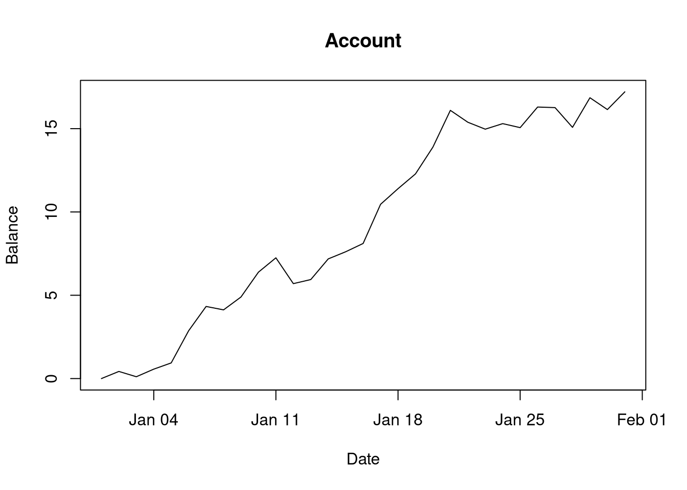
And there’s so much more we could start doing with this construct, such as
writing functions to read transactions and form accounts from CSV files, extend
the generic function as.account(), add an as.transaction() generic functions
and give it methods, etc. We should end the lecture here, though, as we now have
a sensible and functioning class system, which is what we wanted.