Lecture 7
Statistical Intervals
A statistical interval is an interval computed using a sample intended to capture some aspect of the population with some user-specified probability. In this lecture I will discuss some statistical intervals and demonstrate how to compute these intervals in R. When discussing intervals, remember that these include bounds, which is viewed as an interval with one end point being infinite.
Every statistics student encounters confidence intervals and statistics instructors drill students on what the proper interpretation of a confidence interval is. Statisticians care so much about the interpretation of the confidence interval because not only is the wrong interpretation simply wrong, there probably is another interval with the mistaken interpretation that is computed differently from the confidence interval. Here we see some of those other intervals.
Confidence Intervals
Every statistics student should learn how to compute the most common statistical interval: the confidence interval. A \(100C\%\) confidence interval (CI) for some parameter \(\theta\) is an interval such that the probability the interval captures the unknown parameter \(\theta\) when computed from a random sample is \(C\). You should already know how to compute confidence intervals for many contexts, and I will not repeat the discussion here.
Credible Intervals
The Bayesian \(100C\%\) credible interval is an interval such that the probability a population parameter \(\theta\) (here viewed as a random variable of its own) is a specified \(C\). Note that this is not the same interpretation as the confidence intervals, with the subtle difference being that for credible intervals \(\theta\) is viewed as random while for confidence intervals \(\theta\) is fixed and non-raondom, so talking about the “probability” the parameter is in a fixed interval doesn’t make sense (it’s either 1 or 0 depending on whether the parameter is or is not in the interval, though the researcher doesn’t know which is the case).
Computing Bayesian credible intervals requires adopting the Bayesian prior/posterior mindset that goes beyond the scope of this course, so I will not discuss these intervals. Furthermore, Bayesians will compute all of the following intervals differently than the frequentists, so we will ignore Bayesianism from now on.
Prediction Intervals
A \(100C\%\) prediction interval (PI) is an interval such that, if the interval is computed from a random sample \(X_1, \ldots, X_n\), the probability the interval includes the observation \(X_{n+1}\) is \(C\). In short, it’s an interval that predicts where a future observation will appear based on existing observations. Contrast this with CIs which only try to describe the uncertainty associated with the value of a parameter \(\theta\); CIs predict nothing.
Two comments on PIs: first, distributional assumptions matter more to PIs than to CIs. Asymptotic theory allows us to approximate distributions of statistics with some limiting distribution (for example, approximate the distribution of the sample mean with the Normal distribution), but since we’re concerned with the behavior of a single observation, we can’t neglect that observation’s distribution and substitute a limiting distribution like we could with a statistic’s distribution. Second, while prediction intervals can narrow as we collect more data, these intervals don’t “go to zero,” unlike confidence intervals, since an individual observation always has some natural variation not going to zero that must be accounted for.
Let’s start, for instance, with constructing a prediction interval for an observation from a Normal distribution with known standard deviation \(\sigma\). Throughout this lecture assume data is i.i.d.. Then \(\bar{X} = \frac{1}{n} \sum_{i = 1}^n X_i \sim N\left(\mu, \frac{\sigma}{\sqrt{n}}\right)\). Also, \(X_{n + 1} \sim N(0, \sigma)\), and since \(\bar{X}\) and \(X_{n + 1}\) are independent of each other, \(X_{n + 1} - \bar{X} \sim N\left(0, \sigma\sqrt{1 + \frac{1}{n}}\right)\). Thus we can say
\[\frac{X_{n + 1} - \bar{X}}{\sigma\sqrt{1 + \frac{1}{n}}} \sim N(0, 1).\]
We can then form an equal-tail interval by noticing:
\[P\left(-z^* \le \frac{X_{n + 1} - \bar{X}}{\sigma\sqrt{1 + \frac{1}{n}}} \le z^*\right) = P\left(\bar{X} - z^* \sigma \sqrt{1 + \frac{1}{n}} \le X_{n + 1} \le \bar{X} + z^* \sigma \sqrt{1 + \frac{1}{n}}\right) = C\]
where \(z^* = z_{1 - C/2}\). In short, the equal-tailed PI is \(\bar{x} \pm z^* \sigma \sqrt{1 + \frac{1}{n}}\).
Suppose that \(\sigma\) is not known. The resulting calculation is similar to that listed above, and the resulting interval is \(\bar{x} \pm t^* s \sqrt{1 + \frac{1}{n}}\), where \(s\) is the sample standard deviation and \(t^* = t_{n - 1,1 - C/2}\) is the corresponding critical value of the \(t\)-distribution with \(n - 1\) degrees of freedom.
Below is a function for computing the prediction interval for Normally distributed data. It also allows for one-sided intervals, and uses an interface resembling \(t\)-test.
pi_norm <- function(x, conf.level = 0.95, alternative = "two.sided") {
  alpha <- 1 - conf.level
  n <- length(x)
  xbar <- mean(x)
  err <- sd(x) * sqrt(1 + 1 / n)
  crit <- switch(alternative,
                 "two.sided" = qt(alpha / 2, df = n - 1, lower.tail = FALSE),
                 "less" = -qt(alpha, df = n - 1, lower.tail = FALSE),
                 "greater" = qt(alpha, df = n - 1, lower.tail = FALSE),
                 # Below is the "default" switch, triggered if none of the above
                 stop("alternative must be one of two.sided, less, greater"))
  interval <- switch(alternative,
                     "two.sided" = c(xbar - crit * err, xbar + crit * err),
                     "less" = c(xbar + crit * err, Inf),
                     "greater" = c(-Inf, xbar + crit * err),
                     stop("How did I get here?"))
  attr(interval, "conf.level") <- conf.level
  interval
}
Let’s demonstrate by predicting the weight of a cabbage. The data set cabbages
(MASS) contains data from a cabbage field trial (in kilograms). Here I
collect the weights of cabbages from one cultivator.
library(MASS)
cabbage_weight <- subset(cabbages, subset = Cult == "c39")$HeadWt
qqnorm(cabbage_weight)
qqline(cabbage_weight)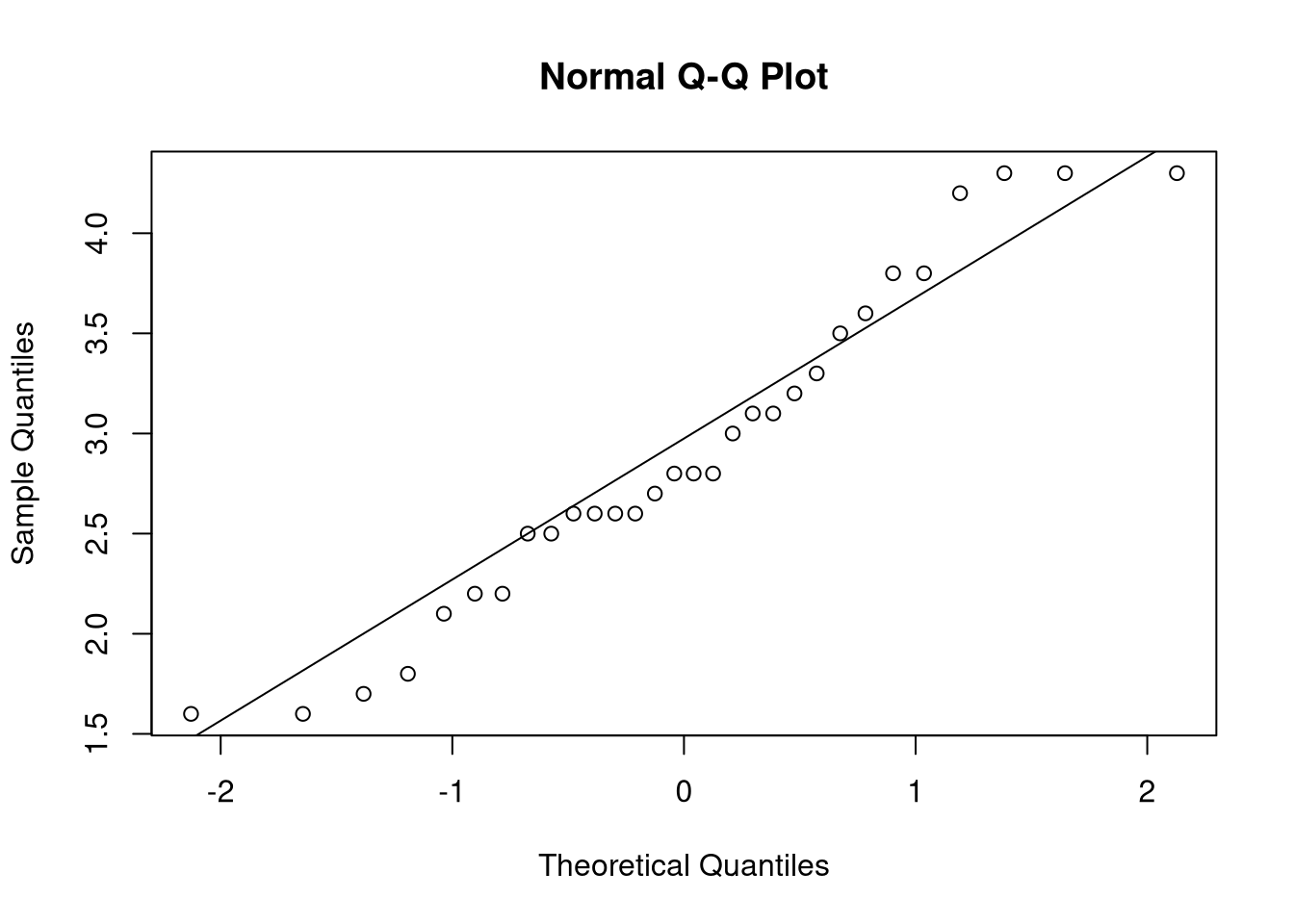
## [1] 1.516780 4.296554
## attr(,"conf.level")
## [1] 0.9
The procedure above, though, is for Normal data. It would never be appropriate to use it for non-Normal data, not even for large sample sizes. So what should we do when our data is not Normally distributed? We have two options:
- If we know the distribution the data came from, we should use an interval designed for that distribution. This is the parameteric approach.
- Use a procedure that assumes very little about the distribution. This is the non-parametric approach.
Computing nonparametric intervals can be done if one assumes the data was drawn from a continuous distribution (it can be done if this not true too but the math is much harder due to the need to account for ties) using the procedure listed here. These intervals are not exact prediction intervals since you may not be able to get an interval for the exact confidence level specified, but they involve few assumptions and we should be able to get close to our desired confidence level. These intervals use the order statistics of the data for their bounds.
The function below can conservatively estimate a prediction interval using a suggested confidence rate. (Only two-sided intervals are allowed by this code.)
no_param_pi <- function(x, conf.level = 0.95) {
  n <- length(x)
  x <- sort(x)
  j <- max(floor((n + 1) * (1 - conf.level) / 2), 1)
  conf.level <- (n + 1 - 2 * j)/(n + 1)
  interval <- c(x[j], x[n + 1 - j])
  attr(interval, "conf.level") <- conf.level
  interval
}
Notice the result of the following:
## [1] -1.959003  2.080691
## attr(,"conf.level")
## [1] 0.95005
The confidence level is slightly higher than the specified 95% but close enough; being lower can happen if there’s not enough data. Furthermore, the resulting prediction interval is close to the interval \((-2, 2)\); recall that the probability that a Normal random variable is within two standard deviations of its mean is roughly 95%, so this interval appears to function as it should.
Here we use it on the cabbage data:
## [1] 1.6 4.3
## attr(,"conf.level")
## [1] 0.9354839
Due to the limitations of the data set, we don’t get a 95% confidence interval; the procedure was forced to just use the maximum and the minimum of the data set as the prediction interval. Nevertheless, it’s close to a 95% interval.
Replication Intervals
Prediction intervals need not be just for a single observation; they could be for any quantity we estimate from future data. For example, we could compute a prediction interval for a future sample mean, of any sample size. When we set the sample size of the future sample mean equal to the sample size of the computed sample mean, I like to call the resulting prediction interval a \(100C\%\) replication interval (RI) since this interval can be interpreted as an interval attempting to capture the value of sample means in replication studies.
Let’s revisit again the Normal case. Let \(\bar{X}_{1,n} = \frac{1}{n}\sum_{i = 1}^n X_i\) represent the observed sample mean and \(\bar{X}_{2,m} = \frac{1}{m} \sum_{i = n + 1}^{n + m} X_i\) the future sample mean for a sample of size \(m\); both of these are treated as random variables, but to construct the interval we will be computing \(\bar{X}_{1,n}\). Since \(\bar{X}_{1,n} \sim N\left(\mu, \frac{\sigma}{\sqrt{n}} \right)\) and \(\bar{X}_{2,m} \sim N\left(\mu, \frac{\sigma}{\sqrt{m}} \right)\) and the two random variables are independent, then
\[\frac{\bar{X}_{1,n} - \bar{X}_{2,m}}{\sigma \sqrt{\frac{1}{n} + \frac{1}{m}}} \sim N(0,1).\]
And in fact the distributional logic developed above applies to this random variable, so we can get a confidence interval even when \(\sigma\) is not known, and obtain the interval \(\bar{x} \pm t^* s \sqrt{\frac{1}{n} + \frac{1}{m}}\) for predicting the value of \(\bar{X}_{2,m}\), with \(t^*\) as before. In fact, if we say \(m = n\), then our interval will be \(\bar{x} \pm \sqrt{2} t^* \frac{s}{\sqrt{n}}\).
Since these intervals are based on the behavior of averages, we can say not only that these intervals will go to zero as we increase our sample sizes \(m\) and \(n\), but also that the intervals should work well regardless of the underlying data distribution if both \(m\) and \(n\) are sufficiently large. These are unlike the earlier prediction intervals, but as with confidence intervals, this is because the objects under study are averages.
Below is a function for computing these replication intervals.
repint <- function(x, m = length(x), conf.level = 0.95,
                   alternative = "two.sided") {
  alpha <- 1 - conf.level
  n <- length(x)
  xbar <- mean(x)
  err <- sd(x) * sqrt(1 / m + 1 / n)
  crit <- switch(alternative,
                 "two.sided" = qt(alpha / 2, df = n - 1, lower.tail = FALSE),
                 "less" = -qt(alpha, df = n - 1, lower.tail = FALSE),
                 "greater" = qt(alpha, df = n - 1, lower.tail = FALSE),
                 # Below is the "default" switch, triggered if none of the above
                 stop("alternative must be one of two.sided, less, greater"))
  interval <- switch(alternative,
                     "two.sided" = c(xbar - crit * err, xbar + crit * err),
                     "less" = c(xbar + crit * err, Inf),
                     "greater" = c(-Inf, xbar + crit * err),
                     stop("How did I get here?"))
  attr(interval, "conf.level") <- conf.level
  interval
}
Here we apply the interval to the cabbage data:
## [1] 2.481725 3.331609
## attr(,"conf.level")
## [1] 0.95
Translated into English, we would say that, with 95% confidence, a future mean
in a replication study (using the same sample size) should lie between r round(repint(cabbage_weight)[[1]], digits = 2) and r round(repint(cabbage_weight)[[2]], digits = 2).
Tolerance Intervals
A tolerance interval (TI) is an interval that contains at least \(100K\%\) of the population with \(100C\%\) confidence. Let’s unpack that statement. The objective of the interval is to create an interval that will contain not only a single future observation but \(100K\%\) of all observations (present and future) for some user-selected \(K \in (0, 1)\). We wish to get such an interval with \(100C\%\) confidence, with \(C\) being the user-specified confidence level that’s appeared in the other intervals. This interval, however, will likely be wider than the true population interval that contains \(100K\%\) of population values due to measurement error, and as a result we should say that the resulting interval contains at least \(100K\%\) of the population values with our specified confidence level.
Unlike PIs, TIs are not trying to predict a future observation but estimate an interval. They’re interval estimates for intervals. But like PIs, TIs can be highly parametric (with distributional assumptions mattering even for large sample sizes) and should not be expected to go to zero for large sample sizes since the underlying interval they’re trying to capture isn’t length zero itself.
The R package tolerance provides functions for computing both parametric and
nonparametric tolerance intervals. For Normal data, we can use the function
normtol.int(). Let’s demonstrate by computing a tolerance interval for cabbage
weight, requiring that the interval capture 90% of cabbage weights. We will make
this a 99% confidence interval.
##   alpha   P    x.bar 2-sided.lower 2-sided.upper
## 1  0.01 0.9 2.906667     0.9813193      4.832014
(Note the parameter alpha and P, which correspond to \(1 - C\) and \(K\) in the
above presentation, respectively.) Additionally, we can compute nonparametric
TIs using the function nptol.int(). Like with nonparametric PIs, nonparametric
TIs depend heavily on sample quantiles. (This is in fact an important theme in
nonparametric statistics in general.)
##   alpha   P 2-sided.lower 2-sided.upper
## 1  0.01 0.9           1.6           4.3