Lecture 4
One-Way Analysis of Variance (ANOVA)
Procedures such as the two-sample \(t\)-test exist to compare the means of two distinct populations. But what if we want to compare the means of more than just two populations? When doing so, we often wish to discern:
- whether there is a difference in the means of any of the populations’ means; and
- if there is a difference, which means are different.
A naïve first attempt would perform two-sample \(t\)-tests for every combination of two populations. If there are \(K\) populations, there would be \({K \choose 2}\) tests. Aside for there being many separate tests (and thus a lot of work), when one conducts many tests like this, the chances of making a Type I error on any test are high, often much higher than the specified Type I error rate \(\alpha\). The Bonferroni correction would suggest we divide the significance level by the number of tests done, thus rejecting one of the null hypotheses if the \(p\)-value drops below \(\alpha/{K \choose 2}\). This correction, however, is quite drastic, perhaps too conservative.
Another solution, at least for determining whether any of the means are different, is to perform what’s known as a “overall” test. In this case, it would determine whether any of the means are different from each other. Depending on the result of the overall test, we would then look to determine which means differ. (If the test does not reject the null hypothesis of no difference we would not proceed with a detailed analysis.)
Analysis of variance (ANOVA) is a statistical procedure looking to address the first issue: whether there is a difference in means among the populations. Later we will look at the other issue.
Suppose there are \(K\) populations; thus, there are \(K\) means, \(\mu_1, \mu_2, \cdots, \mu_K\). ANOVA seeks to decide between:
\[H_0: \mu_1 = \cdots = \mu_K = \mu\]
\[H_A: \text{ there exists } i, j \text{ s.t. } \mu_i \neq \mu_j\]
However, the ANOVA procedure is seen as doing more than just deciding between two hypotheses. In fact, we’re estimating the statistical model:
\[x_{ik} = \mu_k + \epsilon_{ik}\]
where \(i \in \{1,\ldots,n_k\}\) and \(n_1 + \cdots + n_K = N\). The model listed above is the one-way ANOVA model, since the populations differ in only one aspect.
ANOVA assumes that for all \(i\) and \(k\), \(\epsilon_{ik} \sim N(0, \sigma^2)\). We call the terms \(\epsilon_{ik}\) the residuals of the model. The normality of the residuals matters for smaller sample sizes, but less so for larger sample sizes. But the assumption of common variance matters a great deal, regardless of sample size. Thus we must always check it. Statisticians often use box plots to judge whether the common variance assumption is appropriate.
Let \(\bar{x}_k = \frac{1}{n_k} \sum_{i = 1}^{n_k} x_{ik}\) and \(\bar{x}_{\cdot} = \frac{1}{N} \sum_{k = 1}^K \sum_{i = 1}^{n_k} x_{ik}\) \(SSE = \sum_{k = 1}^K \sum_{i = 1}^{n_k} (x_{ik} - \bar{x}_k)^2\) and \(SSTr = \sum_{k = 1}^K (\bar{x}_k - \bar{x}_{\cdot})^2\). Let \(\nu_{n} = K - 1\) and \(\nu_{d} = N - K\) be the numerator and denominator degrees of freedom, respectively. Then the ANOVA test statistic is:
\[f = \frac{SSE/\nu_{n}}{SSTr/\nu_{d}}\]
The distribution of \(f\) if \(H_0\) is true is the \(F\)-distribution \(F_{\nu_{n}, \nu_{d}}\) distribution, the \(F\) distribution with numerator degrees of freedom \(\nu_{n}\) and denominator degrees of freedom \(\nu_{d}\). The \(p\)-value is \(P(F_{\nu_n, \nu_d} > f)\).
A number of R functions can perform ANOVA, particularly oneway.test(),
aov(), and lm().
oneway.test()
Consider the iris data set. Due to the assumption that the populations have a
common variance, we should check with a boxplot whether the assumption seems
plausiable.
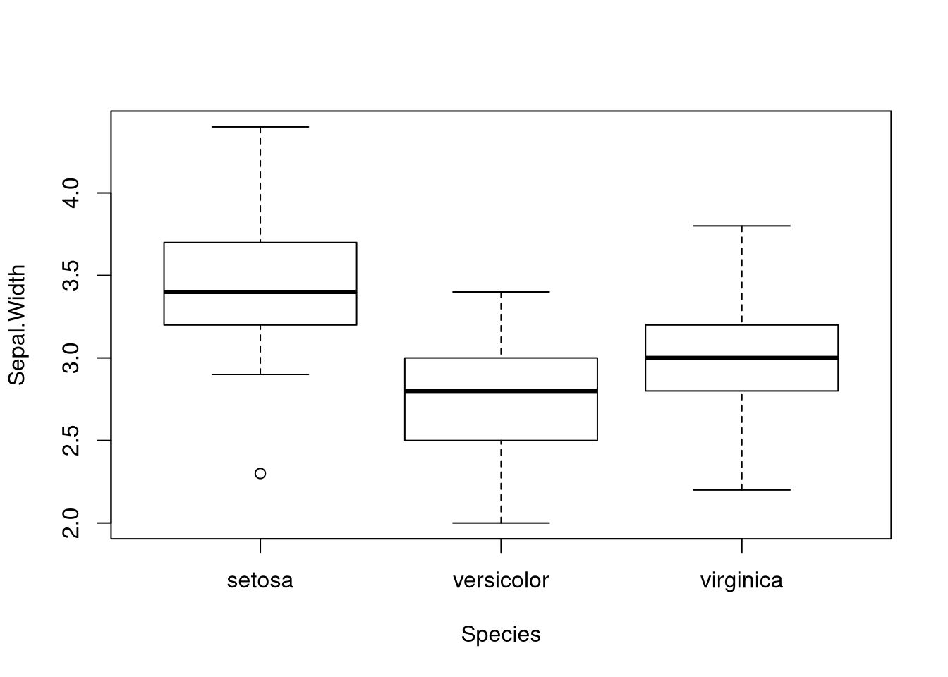
The spread of the data sets are similar; furthermore, the boxplot does suggest
that there could be a difference in means. We instruct oneway.test() to
perform ANOVA via a command resembling oneway.test(x ~ f, data = d), where x
is the variable we test, f identifies the populations, and d is a data frame
containing the variables x and f (in long-form format). Note that x must
be numeric and f must be a factor variable. This holds throughout the
lecture.
##
##  One-way analysis of means (not assuming equal variances)
##
## data:  Sepal.Length and Species
## F = 138.91, num df = 2.000, denom df = 92.211, p-value < 2.2e-16
aov()
aov() performs ANOVA but is more general purpose and tends to produce output
resembling that from other statistics programs. The call to aov() is similar
to the call to oneway.test().
## Call:
##    aov(formula = Sepal.Length ~ Species, data = iris)
##
## Terms:
##                  Species Residuals
## Sum of Squares  63.21213  38.95620
## Deg. of Freedom        2       147
##
## Residual standard error: 0.5147894
## Estimated effects may be unbalanced## Df Sum Sq Mean Sq F value Pr(>F)
## Species 2 63.21 31.606 119.3 <2e-16 ***
## Residuals 147 38.96 0.265
## ---
## Signif. codes: 0 '***' 0.001 '**' 0.01 '*' 0.05 '.' 0.1 ' ' 1lm()
ANOVA is understood as being a particular instance of a linear model. Linear
models will be discussed later, but for now we can see how lm(), the primary
function for estimating linear models, can be used for estimating the ANOVA
model parameters and performing the ANOVA test.
When using lm(), the call is lm(x ~ f - 1, data = d).
##
## Call:
## lm(formula = Sepal.Length ~ Species - 1, data = iris)
##
## Coefficients:
##     Speciessetosa  Speciesversicolor   Speciesvirginica
## 5.006 5.936 6.588##
## Call:
## lm(formula = Sepal.Length ~ Species - 1, data = iris)
##
## Residuals:
## Min 1Q Median 3Q Max
## -1.6880 -0.3285 -0.0060 0.3120 1.3120
##
## Coefficients:
## Estimate Std. Error t value Pr(>|t|)
## Speciessetosa 5.0060 0.0728 68.76 <2e-16 ***
## Speciesversicolor 5.9360 0.0728 81.54 <2e-16 ***
## Speciesvirginica 6.5880 0.0728 90.49 <2e-16 ***
## ---
## Signif. codes: 0 '***' 0.001 '**' 0.01 '*' 0.05 '.' 0.1 ' ' 1
##
## Residual standard error: 0.5148 on 147 degrees of freedom
## Multiple R-squared: 0.9925, Adjusted R-squared: 0.9924
## F-statistic: 6522 on 3 and 147 DF, p-value: < 2.2e-16We should interpret the results found here as only an estimate of the aforementioned ANOVA model. We should not read anything into the statistical tests performed. The reason why is because effectively all that’s being done is testing whether the means of any of the populations are zero, which generally isn’t of interest in this context.
The above command estimated the aforementioned ANOVA model verbatim, but different formulations of the ANOVA model exist. For instance, we could say:
\[x_{i1} = \beta_1 + \epsilon_{i1}\]
\[x_{ik} = \beta_1 + \beta_k + \epsilon_{ik}\]
We interpret \(\mu_1 = \beta_1\) and \(\mu_k = \beta_1 + \beta_k\), or \(\beta_k = \mu_k - \mu_1\). We would then rewrite our hypotheses as:
\[H_0: \beta_2 = \cdots = \beta_K = 0\]
\[H_A: \beta_k \neq 0 \text{ for some } k\]
The lm() call lm(x ~ f, data = d) estimates the parameters of this model and
perform the ANOVA test.
##
## Call:
## lm(formula = Sepal.Length ~ Species, data = iris)
##
## Coefficients:
##       (Intercept)  Speciesversicolor   Speciesvirginica
## 5.006 0.930 1.582##
## Call:
## lm(formula = Sepal.Length ~ Species, data = iris)
##
## Residuals:
## Min 1Q Median 3Q Max
## -1.6880 -0.3285 -0.0060 0.3120 1.3120
##
## Coefficients:
## Estimate Std. Error t value Pr(>|t|)
## (Intercept) 5.0060 0.0728 68.762 < 2e-16 ***
## Speciesversicolor 0.9300 0.1030 9.033 8.77e-16 ***
## Speciesvirginica 1.5820 0.1030 15.366 < 2e-16 ***
## ---
## Signif. codes: 0 '***' 0.001 '**' 0.01 '*' 0.05 '.' 0.1 ' ' 1
##
## Residual standard error: 0.5148 on 147 degrees of freedom
## Multiple R-squared: 0.6187, Adjusted R-squared: 0.6135
## F-statistic: 119.3 on 2 and 147 DF, p-value: < 2.2e-16Finding the Differences
Rejecting the null hypothesis of no difference provides useful information; we know that at least some of the population means are different. However, we also need to determine which means are different, and by how much they differ.
One idea is to compute confidence intervals for differences in means and see which intervals include 0. Any intervals not including zero suggest that the corresponding two populations differ in their means. But if we compute \(t\) confidence intervals as we have done before, then we run into the same multiple hypothesis testing problem we had before. Again, we could look to the Bonferroni correction for guidance, but the original problem of being perhaps too conservative still stands.
A less conservative approach is the Tukey honest significant difference approach. With this approach, a single Type I error rate \(\alpha\) is chosen to represent the probability of any rejection of the null hypothesis of no difference being an error. Then for every pair of populations we compute a confidence interval for the difference in means. We can then use these intervals to determine by how much means of different populations differ.
Recall the object res above formed by a call to aov(). This object is of
class aov and the function TukeyHSD() can accept it as an argument.
TukeyHSD() can then compute the desired confidence intervals.
Let’s demonstrate:
##   Tukey multiple comparisons of means
##     95% family-wise confidence level
##
## Fit: aov(formula = Sepal.Length ~ Species, data = iris)
##
## $Species
##                       diff       lwr       upr p adj
## versicolor-setosa    0.930 0.6862273 1.1737727     0
## virginica-setosa     1.582 1.3382273 1.8257727     0
## virginica-versicolor 0.652 0.4082273 0.8957727     0
The printed output is certainly informative but plots are nice to have. Fortunately plotting these intervals is also easy.
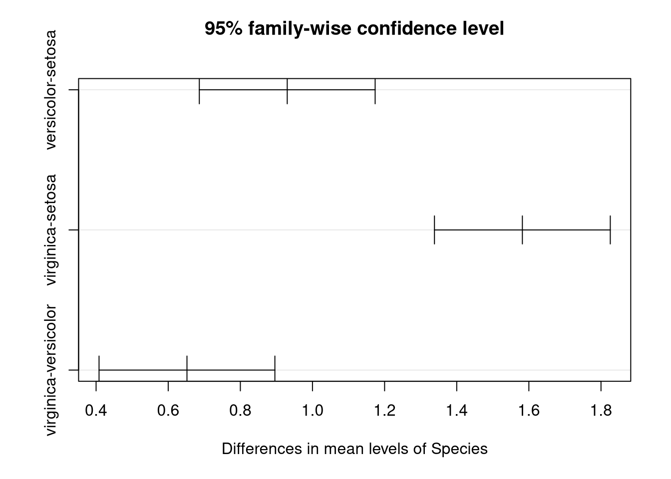
We see that 0 is in none of these intervals. This means that there’s significant evidence that every pair of population means are different, with virginica and setosa flowers having the greatest difference in sepal length and versicolor and virginica the least difference.
There are of course parameters we can set if we want, say, different confidence levels. See the function documentation for more details.