Lecture 12

Nonparametric Statistics

Nonparametric statistics concern statistical inference while making few assumptions about the underlying distribution of the data. Note that this does not mean there are no assumptions about the data; rather, it means we are generally not assuming that the data comes from specific family of distributions. Common assumptions for nonparametric methods are assumptions such as:

The data was drawn from a continuous (i.e. not discrete) distribution.
The distribution from which the data was drawn is symmetric.

Throughout this lecture the first assumption is generally assumed; these methods don’t work as well with discrete data as they do with continuous data. The second assumption may be assumed for certain tests.

Nonparametric methods’ commonly work with the quantiles of the data. Quantities such as the mean or variance may or may not exist for certain distributions. However, quantiles or generalized notions of quantiles can always be defined for any random variable, and for continuous random variables a unique number can be assigned to every quantile. Since quantiles always exist, we can always perform inference for them while making weak assumptions about the data.

Some will view a parametric test such as the sign test, sign-rank test, or the Wilcoxon rank-sum test as equivalent to their parametric cousins such as the \(t\)-test. This is not true since the nonparametric tests generally check quantiles such as the median while \(t\)-tests and \(z\)-tests are tests for the mean. (Granted, the mean and median of the Normal distribution or any symmetric distribution are the same, but in general they are not necessarily the same.) If the research question at hand is specifically for the mean and the data is not assumed to be symmetric, then these nonparametric tests are inappropriate. The reverse is also true; the \(z\)-test should not be used for inference about the median when the data is not symmetric (the \(t\)-test is automatically inappropriate due to non-Normality, but it’s equivalent to the \(z\)-test for large sample sizes).

Sign Test

Let \(q_p\) be the \(100p^{\text{th}}\) percentile of the data; automatically \(q_{0.5}\) is the median of the data. We wish to decide between the hypotheses:

\[H_0: q_p = q_{p0}\]

\[H_A: \begin{cases} q_p > q_{p0} \\ q_p \neq q_{p0} \\ q_p < q_{p0} \end{cases}\]

Let’s continue this discussion but specifically for the median. In order for a number to be the median of a random variable, the probability that the random variable exceeds that number needs to be 0.5. So if \(q_{p0}\) with \(p = 0.5\) were in fact the median, then \(P(X_i > q_{p0}) = p = 0.5\). If the true median was not \(q_{p0}\) though this would not be true. If in fact the true median were greater than \(q_{p0}\) then \(P(X_i > q_{p0}) > p = 0.5\). The converse could also be said; if the true median were less than \(q_{p0}\) then \(P(X_i > q_{p0}) < p = 0.5\). This suggests that what we should be tracking is whether an observation in the sample exceeds \(q_{p0}\) or not. (If an observation exactly equals \(q_{p0}\), delete it.)

If \(T\) is a statistic that counts the number of times an observation exceeds \(q_{p0}\) then the if the null hypothesis is true the distribution of this statistic is known; it counts the number of times the median is exceeded (a “success”) or not (a “failure”), and thus follows a \(\text{Bin}(n, p)\) distribution. If the alternative hypothesis states that the true median is greater than \(q_{p0}\) then large \(T\) would be evidence in favor of the alternative; this would determine how we compute \(p\)-values. Similar statements would be made for the other possible alternative hypotheses. Ultimately the test reduces to a test for population proportion, where the original continuous data is converted to binary data tracking whether the median under the null hypothesis was exceeded or not; hence the term “sign test” since we’re tracking the sign of \(X_i - q_{p0}\).

The function below implements the sign test.

sign.test <- function(x, q = 0, p = 0.5, alternative = "two.sided") {
  res <- list()
  res$data.name <- deparse(substitute(x))
  res$estimate <- c("quantile" = quantile(x, p)[[1]])
  x <- x[x != q]  # Delete observations matching q exactly
  res$method <- "Sign Test"
  res$parameter <- c("p" = p)
  res$alternative <- alternative
  res$null.value <- c("quantile" = q)
  res$statistic <- c("T" = sum(x > q))
  n <- length(x)
  res$p.value <- binom.test(res$statistic, n, p = 1 - p,
                            alternative = alternative)$p.value
  class(res) <- "htest"
  res
}

We will demonstrate its use on simulated data.

(x <- rcauchy(10, location = 3, scale = 2))  # Cauchy distributed; t-test won't

##  [1]  2.832702  2.089755 -5.012347  2.581298  1.853454 -6.199046 92.839383
##  [8]  3.033817  1.402005  6.544141

                                             # work
sign.test(x, q = 3)

## 
##  Sign Test
## 
## data:  x
## T = 3, p = 0.5, p-value = 0.3438
## alternative hypothesis: true quantile is not equal to 3
## sample estimates:
## quantile 
## 2.335527

sign.test(x, q = 2, alternative = "greater")

## 
##  Sign Test
## 
## data:  x
## T = 6, p = 0.5, p-value = 0.377
## alternative hypothesis: true quantile is greater than 2
## sample estimates:
## quantile 
## 2.335527

sign.test(x, q = 2, alternative = "less")

## 
##  Sign Test
## 
## data:  x
## T = 6, p = 0.5, p-value = 0.8281
## alternative hypothesis: true quantile is less than 2
## sample estimates:
## quantile 
## 2.335527

sign.test(x, q = 2, p = 0.25, alternative = "less")  # Testing quartile

## 
##  Sign Test
## 
## data:  x
## T = 6, p = 0.25, p-value = 0.2241
## alternative hypothesis: true quantile is less than 2
## sample estimates:
## quantile 
## 1.514867

Signed-Rank Test

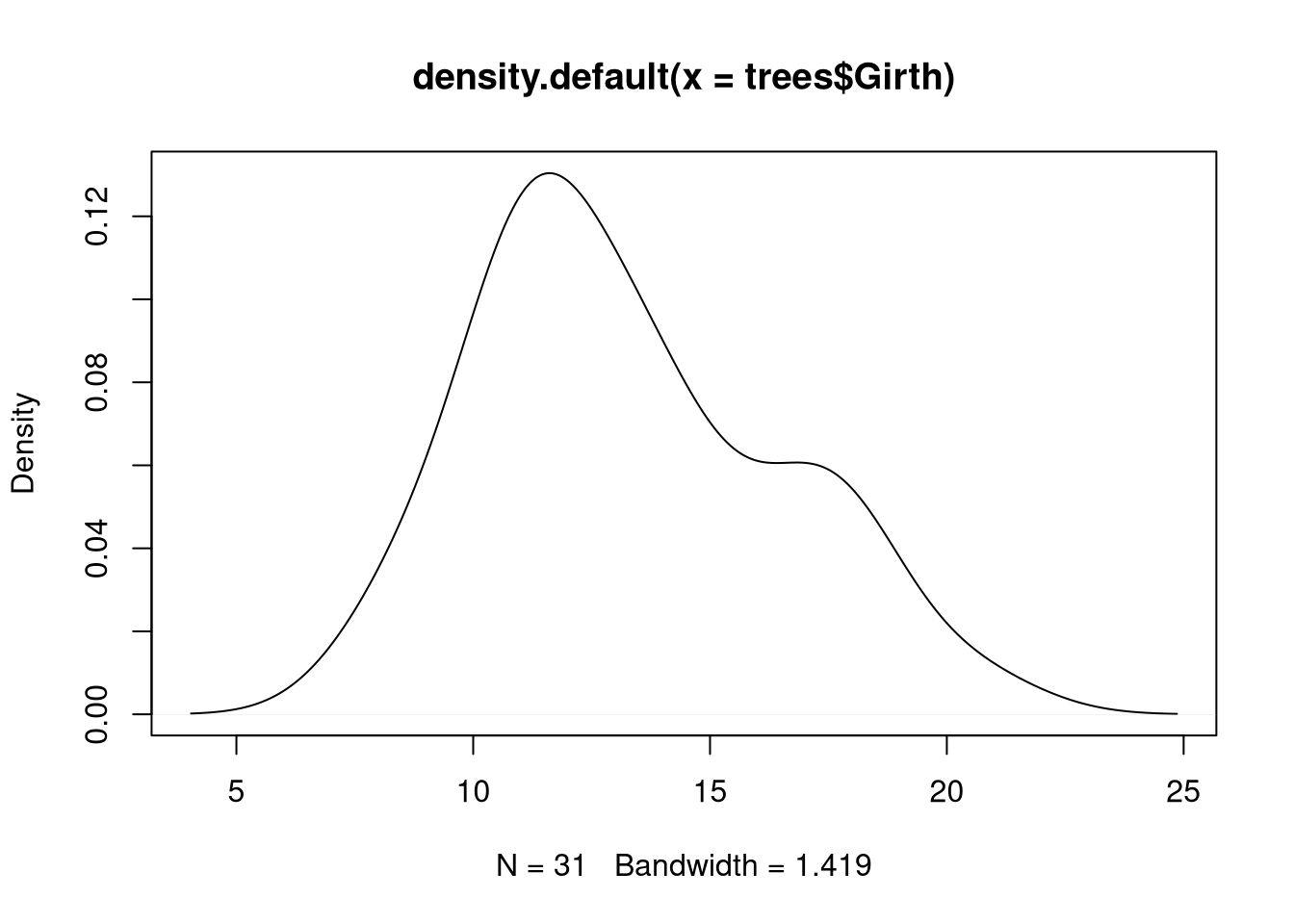
The Wilcoxon signed-rank test is a non-parametric test for the median specifically (as opposed to a general quantile) and is intended for data coming from a symmetric distribution. Before using it, you should check this assumption; look at histograms or density estimates and decide if the data appears reasonably symmetric. The test is intended to have better power than the sign test while not going as far as the \(t\)-test in assuming that the data is Normally distributed. Since we are restricting ourselves to symmetric distributions, the signed-rank test is equivalent to the \(t\)-test when the population has finite and well-defined mean and variance; hopefully the test will have better power than the \(t\)-test, but this is not guaranteed even for non-Normal data (the \(t\)-test is the most powerful test when data is Normally distributed).

We will use the notation \(q_{0.5} = m\). We have the same null and alternative hypotheses as before, but the test statistic not only accounts for whether the data is greater than the median or not (the “signed” part) but also the rank of the data, where one ranks observations by how far away they are from the supposed median (so the closest observation has a rank of 1 and the furthest a rank of \(n\)). The test statstic will be \(T = \sum_{i:x_i > m_0} \text{rank}(\left| x_i - m_0 \right|)\). Suppose that the alternative hypothesis says that the true median is greater than the median under the null hypothesis. Then large \(T\) would serve as evidence against the null hypothesis as observations above the median also tend to be some of the most distant. We can come up with rejection regions for other alternative hypotheses, and the distribution of the statistic under the null hypothesis is known (but not necessarily simple). Thus we can do tests.

The R function for this test is wilcox.test(), with parameters similar to t.test(). Here for example is a demonstration of wilcox.test() to determine whether the median of the girth of trees is 12 or not.

plot(density(trees$Girth))  # Symmetric enough

wilcox.test(trees$Girth, mu = 12)

## Warning in wilcox.test.default(trees$Girth, mu = 12): cannot compute exact
## p-value with ties

## Warning in wilcox.test.default(trees$Girth, mu = 12): cannot compute exact
## p-value with zeroes

## 
##  Wilcoxon signed rank test with continuity correction
## 
## data:  trees$Girth
## V = 323.5, p-value = 0.06263
## alternative hypothesis: true location is not equal to 12

Wilcoxon Rank-Sum Test

The two-sample \(t\)-test helps decide whether the means of two populations are the same or not. The nonparametric equivalent of the two-sample \(t\)-test is the Wilcoxon rank-sum test. The test works for two distributions that are identical except for the location of the median. Let \(m_X\) be the median of one population and \(m_Y\) the median of the other. Then our null hypothesis says:

\[H_0: m_X = m_Y\]

Our alternative is of the form:

\[H_A: \begin{cases} m_X > m_Y \\ m_X \neq m_Y \\ m_X < m_Y \end{cases}\]

The R function for this test is wilcox.test() and takes two data sets. The parameter alternative can be used to set which alternative hypothesis is tested.

# First, let's get the data into separate vectors
split_len <- split(ToothGrowth$len, ToothGrowth$supp)
OJ <- split_len$OJ
VC <- split_len$VC
# Perform statistical test
wilcox.test(OJ, VC, alternative = "greater")

## Warning in wilcox.test.default(OJ, VC, alternative = "greater"): cannot
## compute exact p-value with ties

## 
##  Wilcoxon rank sum test with continuity correction
## 
## data:  OJ and VC
## W = 575.5, p-value = 0.03225
## alternative hypothesis: true location shift is greater than 0