Lecture 11
Two-Way ANOVA
ANOVA was presented as a way to determine if the means of all populations under consideration are the same. One way in which this idea manifests is as testing whether a single set of mutually exclusive treatments have the same effect on subjects or not. Researchers, though, would like to be able to apply multiple classes of treatments to subjects.
For example, let’s consider the ToothGrowth data set.
##    len supp dose
## 1  4.2   VC  0.5
## 2 11.5   VC  0.5
## 3  7.3   VC  0.5
## 4  5.8   VC  0.5
## 5  6.4   VC  0.5
## 6 10.0   VC  0.5
On the one hand, different guinea pigs will be given different types of
supplements: orange juice (OJ) or vitamin C (VC). On the other hand,
different dosages are administered to the guinea pigs, either half, full, or
double dose. We could view these as two different kinds of treatments, which are
not mutually exclusive from each other. In terms of populations, we might say
that while there are different types of populations, we have classes of
population types and there can be overlap of populations when population types
come from different classes.
We first need to ask: are there interactions among treatments? Non-interaction effectively means that the effects of different treatments in some sense “add up”. For example, doubling the dose of vitamin C has relatively the same effect as doubling the dose of orange juice. But interaction would occur if, say, doubling the dose of vitamin C would cause a reduction in tooth growth while doubling the dose of orange juice caused an increase. A model including interactions is harder to interpret than a model without one, though both can be handled.
If we don’t have interactions in the model, then the two-way ANOVA model looks like so:
\[x_{ijk} = \mu_j + \nu_k + \epsilon_{ijk}.\]
In this model \(\mu_j\) is the effect of treatment \(j\) out of \(J\) total treatments in that class while \(\nu_k\) is the effect of treatment \(k\) out of \(K\) total treatments in that class. A two-way ANOVA model with interactions would look like so:
\[x_{ijk} = \mu_j + \nu_k + \gamma_{jk} + \epsilon_{ijk}.\]
The \(\gamma_{jk}\) term is the interaction effect for that combination of populations. Aside from these issues; two-way ANOVA makes the same assumptions as one-way ANOVA: Normally distributed residuals with a constant variance.
We can try to determine if interaction effects exist by using an interaction
plot. Here is an interaction plot for the ToothGrowth data set.
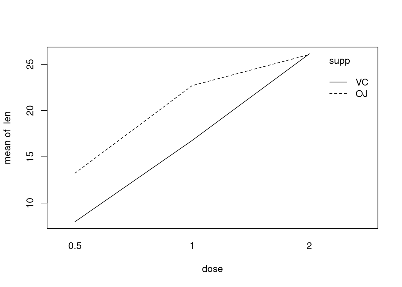
The \(x\)-axis tracks dosage while the \(y\)-axis tracks the mean of the variable
len, the amount of tooth growth in a guinea pig. Different lines are drawn for
supp, or the type of supplement used. We are looking to see if these lines
cross. A crossing of lines suggests that an increase of dosage for one type of
supplement has a different effect than it does for the other dosage. Ideally we
would also have roughly parallel lines. Here there may be a tiny crossing at
double dosage, though not dramatic. The lines are not quite parallel,
unfortunately. It seems that this interaction plot could be interpreted either
way. If one were being conservative, they would likely treat the data as having
interactions, since a model allowing for interactions can cope if there are no
interactions in truth; the opposite direction is harder to say.
Let’s compare with the OrchardSprays data set, which contains the result of an
experiment assessing the potency of different orchard sprays in repelling
honeybees. If one treatment was the type of spray and the other the row position
of where the spray was used, we would get the following interaction plot:
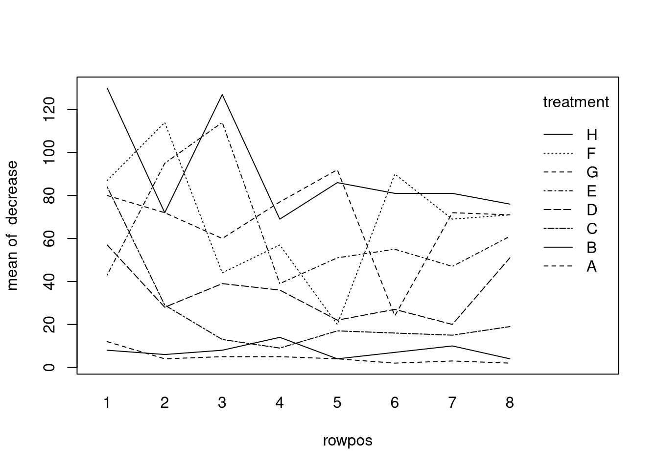 There absolutely are interactions among the factors so a two-way ANOVA model
without interactions certainly would be inappropriate (though I should mention
that a different design was intended for the experiment).
There absolutely are interactions among the factors so a two-way ANOVA model
without interactions certainly would be inappropriate (though I should mention
that a different design was intended for the experiment).
We would like to estimate the two-way ANOVA model, either with or without
interactions. However, we can understand ANOVA, in general, as linear regression
with the regressors being dummy variables. We would have a sequence of dummy
variables for one class of treatments and a sequence of dummy variables for
another class of treatments. Thus we can use lm() to estimate two-way ANOVA
models like so:
##
## Call:
## lm(formula = len ~ supp + as.factor(dose), data = ToothGrowth)
##
## Coefficients:
##      (Intercept)            suppVC  as.factor(dose)1  as.factor(dose)2
##            12.45             -3.70              9.13             15.49
(Notice we have to tell lm() we want dose to be treated as a factor
variable; otherwise, it would be treated as quantitative, which we don’t want.)
The resulting model is phrased in terms of contrasts; the baseline group
consists of guinea pigs that got half a dose of vitamin C. Below we do some
statistics for the model.
##
## Call:
## lm(formula = len ~ supp + as.factor(dose), data = ToothGrowth)
##
## Residuals:
##    Min     1Q Median     3Q    Max
## -7.085 -2.751 -0.800  2.446  9.650
##
## Coefficients:
##                  Estimate Std. Error t value Pr(>|t|)
## (Intercept)       12.4550     0.9883  12.603  < 2e-16 ***
## suppVC            -3.7000     0.9883  -3.744 0.000429 ***
## as.factor(dose)1   9.1300     1.2104   7.543 4.38e-10 ***
## as.factor(dose)2  15.4950     1.2104  12.802  < 2e-16 ***
## ---
## Signif. codes:  0 '***' 0.001 '**' 0.01 '*' 0.05 '.' 0.1 ' ' 1
##
## Residual standard error: 3.828 on 56 degrees of freedom
## Multiple R-squared:  0.7623, Adjusted R-squared:  0.7496
## F-statistic: 59.88 on 3 and 56 DF,  p-value: < 2.2e-16
The \(F\)-test performed can be viewed as a statistical test deciding between the null hypothesis of no treatments having any effect on the response variables and the alternative that at least one treatment has an effect on the response variable. In this case the null hypothesis is rejected; there appears to be some treatment effect, either among the supplement type or the dosage. Furthermore, by examining the results of the tests for the coefficients, just about every possible type of treatment has some effect.
How about allowing for interactions? We can introduce interaction terms like so:
##
## Call:
## lm(formula = len ~ supp * as.factor(dose), data = ToothGrowth)
##
## Coefficients:
##             (Intercept)                   suppVC         as.factor(dose)1
##                   13.23                    -5.25                     9.47
##        as.factor(dose)2  suppVC:as.factor(dose)1  suppVC:as.factor(dose)2
## 12.83 -0.68 5.33##
## Call:
## lm(formula = len ~ supp * as.factor(dose), data = ToothGrowth)
##
## Residuals:
## Min 1Q Median 3Q Max
## -8.20 -2.72 -0.27 2.65 8.27
##
## Coefficients:
## Estimate Std. Error t value Pr(>|t|)
## (Intercept) 13.230 1.148 11.521 3.60e-16 ***
## suppVC -5.250 1.624 -3.233 0.00209 **
## as.factor(dose)1 9.470 1.624 5.831 3.18e-07 ***
## as.factor(dose)2 12.830 1.624 7.900 1.43e-10 ***
## suppVC:as.factor(dose)1 -0.680 2.297 -0.296 0.76831
## suppVC:as.factor(dose)2 5.330 2.297 2.321 0.02411 *
## ---
## Signif. codes: 0 '***' 0.001 '**' 0.01 '*' 0.05 '.' 0.1 ' ' 1
##
## Residual standard error: 3.631 on 54 degrees of freedom
## Multiple R-squared: 0.7937, Adjusted R-squared: 0.7746
## F-statistic: 41.56 on 5 and 54 DF, p-value: < 2.2e-16The results of the new model are more difficult to interpret, both literally and statistically. Additionally, only one potential interaction appears to possibly be statistically significant: the interaction between the vitamin C supplement and the dosage amount.
This begs the question: should we include interaction terms for dosage and supplement or not? So far the results are not particularly conclusive. What we should do is decide whether the coefficients for the interaction terms are statistically different from zero or not. And while we are at it, we should determine whether each type of treatment individually has an effect (not just whether any treatment at all has an effect).
We can do this by using the \(F\) tests for comparing different linear models, with one model being a particular instance of the other, as we did in the last lecture. First we should introduce models representing one-way ANOVA models tracking just supplement type and dosage, like so:
##
## Call:
## lm(formula = len ~ supp, data = ToothGrowth)
##
## Coefficients:
## (Intercept)       suppVC
## 20.66 -3.70##
## Call:
## lm(formula = len ~ as.factor(dose), data = ToothGrowth)
##
## Coefficients:
## (Intercept) as.factor(dose)1 as.factor(dose)2
## 10.61 9.13 15.49Then we compare the model that includes terms for both supplement and dosage to one of these two models. If adding additional terms for another treatment have non-zero coefficients, then the other treatment has an effect on the response variable.
## Analysis of Variance Table
##
## Model 1: len ~ supp
## Model 2: len ~ supp + as.factor(dose)
##   Res.Df    RSS Df Sum of Sq      F    Pr(>F)
## 1     58 3246.9
## 2     56  820.4  2    2426.4 82.811 < 2.2e-16 ***
## ---
## Signif. codes: 0 '***' 0.001 '**' 0.01 '*' 0.05 '.' 0.1 ' ' 1## Analysis of Variance Table
##
## Model 1: len ~ as.factor(dose)
## Model 2: len ~ supp + as.factor(dose)
## Res.Df RSS Df Sum of Sq F Pr(>F)
## 1 57 1025.78
## 2 56 820.43 1 205.35 14.017 0.0004293 ***
## ---
## Signif. codes: 0 '***' 0.001 '**' 0.01 '*' 0.05 '.' 0.1 ' ' 1If we want to see if there are interactions among dosage type and supplement, we can do so by comparing the model with interactions to the one without.
## Analysis of Variance Table
##
## Model 1: len ~ supp + as.factor(dose)
## Model 2: len ~ supp * as.factor(dose)
##   Res.Df    RSS Df Sum of Sq     F  Pr(>F)
## 1     56 820.43
## 2     54 712.11  2    108.32 4.107 0.02186 *
## ---
## Signif. codes:  0 '***' 0.001 '**' 0.01 '*' 0.05 '.' 0.1 ' ' 1
It does seem that there are interactions between dosage and supplement types.
ANOVA models are a particular class of linear model and can be understood as such. ANOVA differs from linear regression mostly in presentation. That said, people care a great deal about presentation, so let’s see how we can perform two-way ANOVA with some of the other functions we’ve seen.
The aov() function we saw earlier is well-equipped for two-way ANOVA, and can
be called basically just like lm(). The advantage to using aov() is that
it’s specifically designed for ANOVA.
## Call:
##    aov(formula = len ~ supp + as.factor(dose), data = ToothGrowth)
##
## Terms:
##                     supp as.factor(dose) Residuals
## Sum of Squares   205.350        2426.434   820.425
## Deg. of Freedom        1               2        56
##
## Residual standard error: 3.82759
## Estimated effects may be unbalanced## Call:
## aov(formula = len ~ supp * as.factor(dose), data = ToothGrowth)
##
## Terms:
## supp as.factor(dose) supp:as.factor(dose) Residuals
## Sum of Squares 205.350 2426.434 108.319 712.106
## Deg. of Freedom 1 2 2 54
##
## Residual standard error: 3.631411
## Estimated effects may be unbalanced