Lecture 2

Environments

Environments are special data structures that are responsible for handling the names of variables and for looking up variables when requested. You have been interacting with environments for as long as you have been using R. Whenever you create a variable in R, what you have actually done is created an object then created a slot in the global environment (the environment where user action in R generally takes place) that points to that object. If an object has no slot in an environment pointing to that object, R automatically destroys it during a process known as garbage collection.

The function ls() lists the objects contained in an environment. By default, it lists what’s in the global environment.

ls()

##  [1] "_Mean.1_"       "%s%"            "%s0%"           "1.Mean_"       
##  [5] "Awesome sauce!" "collector"      "error_obj"      "f_num"         
##  [9] "i"              "idx"            "increment"      "l"             
## [13] "m"              "n"              "new_collector"  "paste_"        
## [17] "s_num"          "stat"           "sum"            "t_num"         
## [21] "u"              "x"              "z.stat"

ls(envir = globalenv())  # globalenv() accesses the global environment

##  [1] "_Mean.1_"       "%s%"            "%s0%"           "1.Mean_"       
##  [5] "Awesome sauce!" "collector"      "error_obj"      "f_num"         
##  [9] "i"              "idx"            "increment"      "l"             
## [13] "m"              "n"              "new_collector"  "paste_"        
## [17] "s_num"          "stat"           "sum"            "t_num"         
## [21] "u"              "x"              "z.stat"

x <- 1
ls()

##  [1] "_Mean.1_"       "%s%"            "%s0%"           "1.Mean_"       
##  [5] "Awesome sauce!" "collector"      "error_obj"      "f_num"         
##  [9] "i"              "idx"            "increment"      "l"             
## [13] "m"              "n"              "new_collector"  "paste_"        
## [17] "s_num"          "stat"           "sum"            "t_num"         
## [21] "u"              "x"              "z.stat"

ls(envir = globalenv())

##  [1] "_Mean.1_"       "%s%"            "%s0%"           "1.Mean_"       
##  [5] "Awesome sauce!" "collector"      "error_obj"      "f_num"         
##  [9] "i"              "idx"            "increment"      "l"             
## [13] "m"              "n"              "new_collector"  "paste_"        
## [17] "s_num"          "stat"           "sum"            "t_num"         
## [21] "u"              "x"              "z.stat"

The function environment() lists the current environment.

environment()

## <environment: R_GlobalEnv>

In fact, we can access objects in environments similarly to how we access objects in lists. However, environments are not just a different kind of list. We’ll get into that in a second; let’s first see how environments have similar syntax to lists. We can create a new environment with the function new.env(). Objects in the environment can be referenced using $, like so:

my_env <- new.env()
my_env$x <- 1
my_env[["y"]] <- 2
my_env[["awesome sauce"]] <- 3

my_env[["x"]] + my_env$y + my_env$`awesome sauce`

## [1] 6

ls(envir = my_env)

## [1] "awesome sauce" "x"             "y"

However, despite these similarities, there are important distinctions between environments and lists, such as objects saved in an environment are unordered; there is no “first” item. So in the above code, my_env[1] and my_env[[1]] make no sense. Names in environments are unique, and environments have reference semantics. Additionally, you don’t remove objects from environments by setting them to NULL, as you would with a list. Instead, you have to use the function rm(), like so:

rm(list = "awesome sauce", envir = my_env)

There are two fundamental ingredients needed for an environment: a frame (which are the name-object bindings demonstrated above) and the environment’s parent environment, which is an environment that “contains” the environment. There is only one environment that does not have a parent: the empty environment (created automatically and referenced with emptyenv()). Otherwise, every environment has a parent. Aside from emptyenv(), two other important environments are the global environment (referenced via globalenv() and represents the environment that the user generally works in) and baseenv() (the environment of the base package).

When we create an environment, we can declare its parent like so:

other_env <- new.env(parent = my_env)
other_env$z <- "great!"
my_env

## <environment: 0x55910d17a400>

parent.env(other_env)  # Find the parent of an environment

## <environment: 0x55910d17a400>

By default, the parent of an environment created via new.env() is the global environment. When using environments as data structures (say, as a substitute for a list), consider making the parent the empty environment.

Due to the parent-child nature of environments, we could say that any environment has a sequence of ancestors, consisting of the parent of a given environment, the parent of the parent environment, and so on. The only environment that does not have a parent is the empty environment. Furthermore, the empty environment is the ultimate ancestor of all environments.

To compare environments, we use a function called identical(); we cannot use ==. I demonstrate use of identical() below:

parent.env(globalenv())

## <environment: package:stats>
## attr(,"name")
## [1] "package:stats"
## attr(,"path")
## [1] "/usr/lib/R/library/stats"

identical(emptyenv(), globalenv())

## [1] FALSE

identical(my_env, other_env)

## [1] FALSE

identical(my_env, my_env)

## [1] TRUE

Functions and Environments

Why does this discussion matter? Users generally are not creating environments. Instead, environments are generated automatically when functions are called. Users don’t notice because those environments are often instantly destroyed when the function completes and terminates. However, this matters when understanding and creating closures.

Consider the following function:

x <- 10
y <- 20
f <- function() {
  x <- 30
  cat("x is", x, "\n")
  cat("y is", y, "\n")
}
f()

## x is 30 
## y is 20

## [1] 10

## [1] 20

x <- 40
y <- 50
f()

## x is 30 
## y is 50

## [1] 40

## [1] 50

What happened here? Here’s a step-by-step breakdown of the above code sequence:

Variables x and y were created in the global namespace with some initial values.
The function f() was defined, then called. When f() was called, a new environment was temporarily created, with the global environment being its parent.
A variable x was defined in the environment where f() operated. This x is distinct from the x that was defined in the global environment, since they were defined in two separate environments. This is the reason why the value of x in the global environment was not changed.
When x was referenced in f(), R first looked inside the active environment, the temporary one created when the function was called. x was found there, so the x that existed in the global environment was ignored. When y was referenced, no y was found in the active environment, so R looked in the parent environment, which was the global environment. A definition for y was found there, and so it was the variable referenced.
We later changed the value of x and y in the global environment. The first temporary environment from when f() was called the first time was destroyed when the function finished its execution. When we called the function a second time, a brand new environment was created, with the global environment as its parent. x was still created in this new environment, with its same value as before. The change to x in the global environment didn’t affect the function’s execution. The reference to y, though, did cause different behavior, since the y referred to in the function was the y that existed in the global environment.

What if we wanted to change the value of a variable in the global environment from the function? We could do so by using <<-, which will only create a variable if no name is found in any of the current environment’s ancestors, and if no reference is found, the variable is created in the global environment. <<- is demonstrated below:

x <- 10
y <- 20
g <- function() {
  x <<- 30
  cat("x is", x, "\n")
  cat("y is", y, "\n")
}
g()

## x is 30 
## y is 20

## [1] 30

## [1] 20

Now this time x was changed in the global environment. This is because when <<- was called, it looked for x in the active environment, didn’t find it, then looked in the parent of the active environment, which was the global environment. It found x there, and modified its value. When x and y were referenced in the function, both of them were from the global environment (before, only y was a global variable).

Namespaces

A namespace is a special environment associated with a package. Each package has its own namespace that is attached to the global environment when the package is loaded. However, thanks to namespaces, we can even reference functions in packages without even loading the package.

We reference objects in namespaces via either :: or :::, using syntax such as namespace::object or namespace:::object. The difference between :: and ::: is that :: only accesses public objects, or objects that the package authors have marked as available to all of R when the package is referenced. ::: accesses all objects in a package, including private ones that the package authors did not intend to make available to other code and probably don’t want to be available. While referencing package objects via ::, referencing via ::: is unsafe and should be avoided.

For example, the function mvrnorm() from the package MASS allows for simulating random variables that are joinly Normal. We can use this function without explicitly loading MASS via :: like so:

MASS::mvrnorm(n = 10, mu = c(1, 1), Sigma = matrix(c(1, 0.5, 0.5, 1), nrow = 2))

##             [,1]      [,2]
##  [1,]  0.6140040 0.4498941
##  [2,]  1.3633067 0.7191522
##  [3,]  1.1062482 0.4535209
##  [4,] -0.8262249 0.1702595
##  [5,]  0.1940201 1.9191629
##  [6,]  1.3518935 0.6685813
##  [7,]  1.1313676 1.5529045
##  [8,]  0.5231649 1.9132617
##  [9,] -0.5563917 0.2959209
## [10,]  0.3515644 0.1049541

Why do namespaces matter? Consider the function sd() which is a function from the packages stats that computes standard deviations. Reading the function’s code reveals that it calls the function var(), also from stats, to compute the standard deviation.

sd

## function (x, na.rm = FALSE) 
## sqrt(var(if (is.vector(x) || is.factor(x)) x else as.double(x), 
##     na.rm = na.rm))
## <bytecode: 0x55910bedef50>
## <environment: namespace:stats>

The following code reveals that both sd() and var() “live” in an environment that is not the global environment.

environment(sd)

## <environment: namespace:stats>

environment(var)

## <environment: namespace:stats>

What if we change var? Will doing so break sd()?

x <- rnorm(10)
var(x)

## [1] 1.058425

sd(x)

## [1] 1.028798

var <- function(x) {10}
var(x)

## [1] 10

sd(x)

## [1] 1.028798

The output of sd() is unchanged. This is because sd() refers to the version of var() that lives in its namespace, and doesn’t care about the version that lives in the global environment. The var() in sd()’s namespace can’t be modified in an active R session; one would have to modify the code of the stats package in order to change var(). Therefore, sd() performs as expected.

If we wanted to go back to the old var(), we could do so via the following code:

var

## function(x) {10}

var <- stats::var
var

## function (x, y = NULL, na.rm = FALSE, use) 
## {
##     if (missing(use)) 
##         use <- if (na.rm) 
##             "na.or.complete"
##         else "everything"
##     na.method <- pmatch(use, c("all.obs", "complete.obs", "pairwise.complete.obs", 
##         "everything", "na.or.complete"))
##     if (is.na(na.method)) 
##         stop("invalid 'use' argument")
##     if (is.data.frame(x)) 
##         x <- as.matrix(x)
##     else stopifnot(is.atomic(x))
##     if (is.data.frame(y)) 
##         y <- as.matrix(y)
##     else stopifnot(is.atomic(y))
##     .Call(C_cov, x, y, na.method, FALSE)
## }
## <bytecode: 0x55910c0436d0>
## <environment: namespace:stats>

Closures

The above discussions about environments may have been enlightening, but the primary motivation was to allow discussion of writing functions that can return closures, which are also functions (the term simply distinguishes a function created by another function from usual functions).

Here’s an example of a function that returns closures:

incrementer <- function(i) {
  function(x) {
    x + i
  }
}

f <- incrementer(2)
class(f)

## [1] "function"

f(1:3)

## [1] 3 4 5

g <- incrementer(200)
g(1:3)

## [1] 201 202 203

Closure constructors can be powerful tools, but to the uninitiated they can be mysterious. Why is it, for example, that both f() and g() remember the value i was set to when they were created?

The answer is environments. When we see what environment the functions “live” in, we discover it’s not the global environment. Instead, these functions still use the “temporary” environments created when the function incrementer() was invoked; these environments were actually not destroyed when the function ended since other functions were created in those environments, then returned, and thus those environments are still needed. We in fact see that the environments the closures use are not the global environment:

environment(incrementer)

## <environment: R_GlobalEnv>

environment(f)

## <environment: 0x55910c470c90>

environment(g)

## <environment: 0x55910c6e84a8>

And in fact we see that the i values from those function calls live on in those environments.

ls(envir = environment(f))

## [1] "i"

environment(f)$i

## [1] 2

environment(g)$i

## [1] 200

These features give closures their true power. For example, we can create functions that remember how many times they were called.

elephant_func <- function() {  # Cuz elephants never forget
  calls <- 0
  function() {
    calls <<- calls + 1
    calls
  }
}

e1 <- elephant_func()
e1()

## [1] 1

e1()

## [1] 2

e1()

## [1] 3

e2 <- elephant_func()
e2()

## [1] 1

e2()

## [1] 2

e1()

## [1] 4

This set of functions may be more difficult to unparse than the examples we saw before, yet the only difference in the logic is that the parent environment of, say, e1()’s execution environment is not the global environment anymore but instead the environment created upon e1()’s birth. This is distinct from the parent environment of any environment created by e2()’s execution.

Here’s one application of closures. Suppose that we want to examine multiple confidence intervals for any given data set and we want an easy interface for doing so. With closures we can create easy interfaces for changing the parameters of confidence intervals, perhaps changing confidence levels or making them one-sided or two-sided. The following code is a function factory implementing this idea:

dat_ci <- function(dat) {
  function(C = 0.95, type = "two.sided") {
    alternative <- switch(type,
      "two.sided" = "two.sided",
      "upper" = "less",
      "lower" = "greater"
    )
    c(t.test(dat, alternative = alternative, conf.level = C)$conf.int)
  }
}

x1 <- rnorm(10)
c1 <- dat_ci(x1)
c1()

## [1] -0.6752207  0.5351377

c1(0.9)

## [1] -0.5604414  0.4203585

c1(0.99)

## [1] -0.9394474  0.7993645

c1(0.99, "upper")

## [1]      -Inf 0.6847582

x2 <- rnorm(10)
c2 <- dat_ci(x2)
c2(0.99)

## [1] -0.2349545  1.1986683

Often in statistics we want to treat a data set as fixed but allow for, say, a parameter, to vary. Closures make doing this easier. Let’s consider, for example, the sum of square errors:

\[SSE(\theta) = \sum_{i = 1}^n (x_i - \theta)^2\]

We want to find $\theta$ that minimizes the sum of square errors; we might call such a $\theta$ a best predictor for an observation, or a good statistic describing the location of $x_i$. Calculus reveals that the value of $\theta$ that minimizes $SSE(\theta)$ is $\theta = \bar{x}$, the sample mean. But let’s see if we can avoid calculus.

We can write a function that produces closures that compute $SSE(\theta)$ for input $\theta$ given a fixed data set. We would like this function to produce a vector of SSEs if given a vector of values of $\theta$. We do this by actually returning a vectorized version of the $SSE(\theta)$ function using the Vectorize() function (which is a functional that returns closures). The final implementation is below:

sse_computer <- function(x) {
  f <- function(t) {
    if (!is.numeric(t) || length(t) > 1) stop("Invalid t")
    sum((x - t)^2)
  }
  Vectorize(f)
}

If we wished to plot $SSE(\theta)$ for a given data set, we can do so via the curve() function, which is a plotting function with an interface friendly to mathematical functions (try curve(exp, -2, 2) if you want a quick demo; this is $e^x$ plotted from $x = -10$ to $x = 10$).

x <- rnorm(20, mean = 10)
sse <- sse_computer(x)
curve(sse, 8, 12)

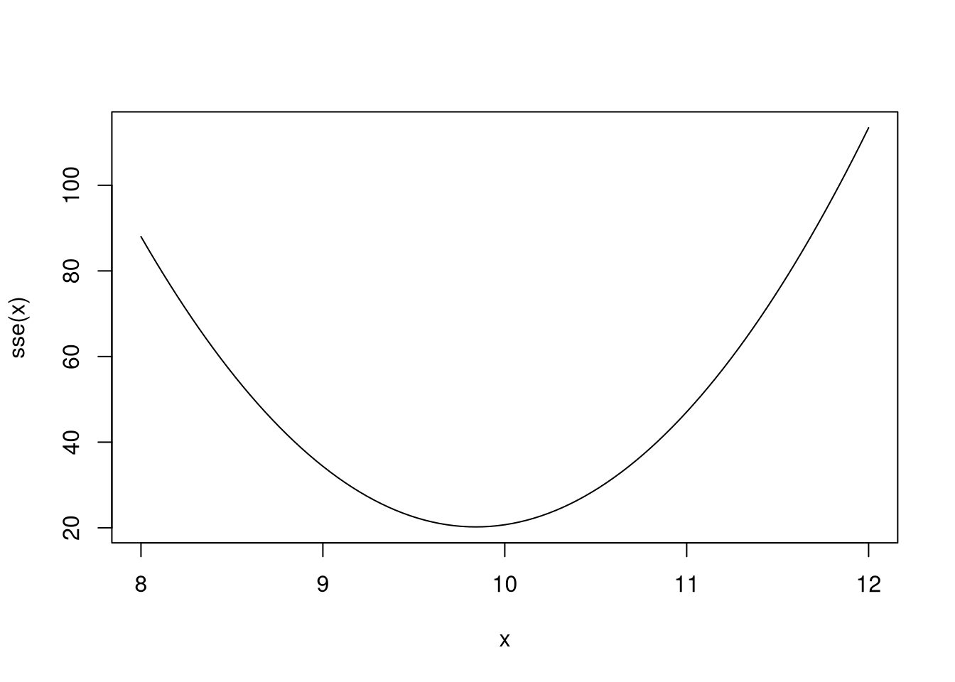
The curve seems to take a minimum near 10 (which is the known mean of the data.) For reference, the mean of the data is 9.8411906. That said, for what value of $\theta$ is $SSE(\theta)$ minimized?

For this we can use the function optimize(), which is a numerical optimizer. The first argument to optimize() is a function to minimize. (If we wish to maximize a function, recall that maximizing $f$ is the same thing as minimizing $-f$. For this reason, optimization literature generally discusses only minimization problems since such problems automatically include maximization.) The second argument is a vector defining the interval over which the function should be minimized. The function then returns a list with elements minimum and objective, with minimum being where the minimum is attained (in our case, the optimal $\theta$) and objective the value of the function at the minimum (here, $SSE(\theta)$).

Optimization here is easy:

optimize(sse, c(-100, 100))

## $minimum
## [1] 9.841191
## 
## $objective
## [1] 20.21141

mean(x)  # For comparison

## [1] 9.841191

These are of course only some uses for closures. I have used them to gain control over random number generation or to write functions that make predictions from fitted models. As the course progresses, look out for more uses of closures (especially after discussing linear models).

Replacement Functions

Consider the following code:

vec <- 1:3
names(vec) <- c("a", "b", "c")
vec

## a b c 
## 1 2 3

How odd is this code? Doesn’t it seem strange that a function call can cause the value of an input to that function to change, simply because of assignment?

Actually, the above code is misleading, for it was not the function names() that was called, but names<-().

names

## function (x)  .Primitive("names")

`names<-`

## function (x, value)  .Primitive("names<-")

A commandment of functional programming is that code should not have side effects. So a function call f(x) should not modify the state of variables outside of f nor should x have its value modified. Following this rule helps make code more easily understood and reasoned about. However, replacement functions such as names<-() test this principle; while technically adhereing to at least the spirit of the rule, it at least seems as if they change the value of their arguments. (That said, one can still reason easily about the state of the program after this function is called due to the presence of the assignment operator to the right of a function call.)

We write replacement functions like we would any other function, with the following restrictions:

Our function name should be wrapped in backticks (like with infix functions) and end with <-.
We must have at least two arguments, which we call x and value, with x coming before value. They correspond to f(x) <- value.
We may have additional arguments, but any additional arguments must be between x and value.
The function must return the modified copy of x.

I present a simple (yet stupid) example below, where the function changes the values of vectors in particular positions:

`modify2<-` <- function(x, value) {
  x[2] <- value
  x
}

x <- 1:10
modify2(x) <- 100
x

##  [1]   1 100   3   4   5   6   7   8   9  10

# With a position argument
`modify<-` <- function(x, pos = 1, value) {
  x[pos] <- value
  x
}

modify(x) <- 20
modify(x, 2) <- -2
x

##  [1] 20 -2  3  4  5  6  7  8  9 10