Lecture 14
Beyond Linear Models
In this section we will explore models that are not linear models, in that they are not linear in their parameters. Recall that linear models are models that take the form:
\[y_i = \beta_0 + \beta_1 x_{1i} + \cdots + \beta_k x_{ki} + \epsilon_i.\]
They either take that form exactly or could take that form after some transformation (commonly a log transformation). Before looking at nonlinear models, make sure that the model is not linear after a transformation. For instance, the model:
\[y_i = \beta_0 x_i^{\beta_1} \epsilon_i\]
is linear in the parameters after taking a log transform:
\[\log(y_i) = \log(\beta_0) + \beta_1 \log(x_i) + \log(\epsilon_i).\]
But the model below is not linear in the parameters:
\[y_i = \beta_0 e^{\beta_1 x_i} + \epsilon_i.\]
We will first talk about a particular nonlinear model: logistic regression. Then we will discuss estimating nonlinear models in general.
Logistic Regression
Suppose \(y_i \in \left\{0, 1\right\}\); that is, \(y_i\) is a Bernoulli random variable. We would like to predict whether \(y_i\) is either 0 or 1 using a set of regressors \(x_1, \ldots, x_k\). We could try using the linear model above, but unfortunately the error terms will not be i.i.d. and won’t even look remotely Normal. Additionally, the resulting model will produce strange “predictions”; we would interpret the model as estimating the probability that \(y_i = 1\) based on \(x_1, \ldots, x_k\), but the model can give probabilities above 1 or below 0. These are undesirable properties that call for a different procedure.
Logisitic regression is a regression procedure that fixes these properties. Let \(\pi_i\) be the probability that \(y_i = 1\). Logistic regression estimates the model
\[\pi_i = \frac{e^{\beta_0 + \beta_1 x_{1i} + \cdots + \beta_k x_{ki} + \epsilon_i}}{1 + e^{\beta_0 + \beta_1 x_{1i} + \cdots + \beta_k x_{ki} + \epsilon_i}} = g(\beta_0 + \beta_1 x_{1i} + \cdots + \beta_k x_{ki} + \epsilon_i).\]
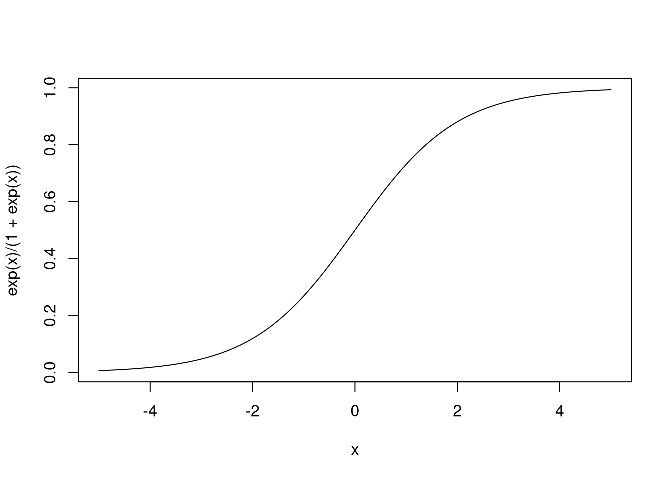
The function \(g(x) = \frac{e^x}{1 + e^x}\) is known as the logistic function, and it only takes values between 0 and 1, and thus can produce probabilities.
Another term for the model produced by logistic regression is logit models.
The predicted values from logistic regression are not 1 or 0 but the probability that the response variable is 1 or 0 given the values of the regressors. If you want to convert these probabilities into predictions, you would perhaps threshold these probabilities so that probabilities above, say, 0.5 will be predictions that \(y_i = 1\) and all others predict \(y_i = 0\).
The coefficients themselves are more difficult to interpret, but they can be interpreted. Recall that if the probability an event \(A\) occurs is \(p\), then the odds that \(A\) occurs is \(\frac{p}{1 - p}\) to 1. It turns out that the logistic regression model can be rewritten as:
\[\ln\left(\frac{\pi_i}{1 - \pi_i}\right) = \beta_0 + \beta_1 x_{1i} + \cdots + \beta_k x_{ki} + \epsilon_i.\]
We call \(\ln\left(\frac{\pi_i}{1 - \pi_i}\right)\) the log-odds that \(y_i = 1\), and so we are estimating a linear model to predict the log-odds that our response variable is 1. We could then say that a unit increase in \(x_{ji}\) predicts that the log-odds will increase by \(\beta_j\), or that the odds will increase by a factor of \(e^{\beta_j}\). (And for what it’s worth, sometimes a logit model is accompanied by a linear model since linear model parameters are easily interpreted.)
Logit models must be estimated numerically, but the good news is that inference
procedures we saw before, including marginal \(t\)-tests and AIC inference, still
hold. In R, the function for estimating logit models is glm(), which can be
understood as meaning “generalized linear model”. glm() can actually estimate
a lot of models, including models where we have specific assumptions about what
the distribution of the response variables are (such as poisson or gamma), and
much can be said about it. Here, though, I will only show how to use it for
logistic regression.
If we want to estimate a logit model, our function call will resemble glm(y ~ x, data = d, family = binomial). The function call is almost identical to
lm(), but we have an additional parameter, family, that identifies the type
of regression model we’re estimating. By default, family = binomial performs
logistic regression.
Let’s demonstrate by building a logit model to predict whether an iris flower is a member of the versicolor species or not. We will use the sepal length, sepal width, petal length, and petal width for our predictions.
(fit <- glm(I(Species == "versicolor") ~ Sepal.Length + Sepal.Width +
            Petal.Length + Petal.Width, data = iris, family = binomial))
##
## Call: glm(formula = I(Species == "versicolor") ~ Sepal.Length + Sepal.Width +
## Petal.Length + Petal.Width, family = binomial, data = iris)
##
## Coefficients:
## (Intercept) Sepal.Length Sepal.Width Petal.Length Petal.Width
## 7.3785 -0.2454 -2.7966 1.3136 -2.7783
##
## Degrees of Freedom: 149 Total (i.e. Null); 145 Residual
## Null Deviance: 191
## Residual Deviance: 145.1 AIC: 155.1##
## Call:
## glm(formula = I(Species == "versicolor") ~ Sepal.Length + Sepal.Width +
## Petal.Length + Petal.Width, family = binomial, data = iris)
##
## Deviance Residuals:
## Min 1Q Median 3Q Max
## -2.1280 -0.7668 -0.3818 0.7866 2.1202
##
## Coefficients:
## Estimate Std. Error z value Pr(>|z|)
## (Intercept) 7.3785 2.4993 2.952 0.003155 **
## Sepal.Length -0.2454 0.6496 -0.378 0.705634
## Sepal.Width -2.7966 0.7835 -3.569 0.000358 ***
## Petal.Length 1.3136 0.6838 1.921 0.054713 .
## Petal.Width -2.7783 1.1731 -2.368 0.017868 *
## ---
## Signif. codes: 0 '***' 0.001 '**' 0.01 '*' 0.05 '.' 0.1 ' ' 1
##
## (Dispersion parameter for binomial family taken to be 1)
##
## Null deviance: 190.95 on 149 degrees of freedom
## Residual deviance: 145.07 on 145 degrees of freedom
## AIC: 155.07
##
## Number of Fisher Scoring iterations: 5## (Intercept) Sepal.Length Sepal.Width Petal.Length Petal.Width
## 1.601165e+03 7.824254e-01 6.101912e-02 3.719701e+00 6.214133e-02## [1] "glm" "lm"glm() produces glm-class objects, which inherit from lm-class objects. So
functions such as predict() or coef() work for these objects, and they have
similar structures.
Nonlinear Models
A nonlinear model is not linear in its coefficients, and many of these models take the form:
\[y_i = f(x_{1i}, \ldots, x_{k1}; \beta_0, \beta_1, \ldots, \beta_r) + \epsilon_i.\]
(Note that \(r\) and \(k\) may be different.) I gave an example of a nonlinear model above, and this class of models is quite general. We still interpret \(\beta_0, \ldots, \beta_r\) as parameters of the model and \(f(\cdots ; \beta_0, \ldots, \beta_r)\) as a function giving predicted values for \(y_i\) since the residuals \(\epsilon_i\) are still assumed to be i.i.d. with mean 0. In fact the least-squares principle still holds since we want to pick \(\hat{\beta}_0, \ldots, \hat{\beta}_r\) that minimize
\[SSE(\hat{\beta}_0, \ldots, \hat{\beta}_r) = \sum_{i = 1}^n \left(y_i - f(x_{1i}, \ldots, x_{ki}; \hat{\beta}_0, \ldots, \hat{\beta}_r)\right)^2.\]
In the case of linear models, the coefficients of the model can be solved for explicitly, perhaps after invoking linear algebra. That is not the case in general and generally one must resort to numerical techniques to estimate nonlinear models. As for what form \(f\) itself takes, that’s a domain-specific problem; there could be a physical or biological model that dictates the form of \(f\), which is known up to the parameters (which we as statisticians then try to estimate).
Numerical optimization procedures/numerical solvers are iterative and generally need a set of starting parameters in order to work. This means that users of these methods need to make an educated guess as to what the true parameters are. Perhaps consider using plots to form guesses as to what the parameter values are, getting parameter values that appear to be “close” to fitting the data. (This is completely subjective, by the way.) Once you have a decent guess at the parameter values, you can then use the numerical procedures to get the proper fit.
The R function for nonlinear least squares estimation is nls(), whose function
calls often take the form nls(formula, data = d, start = v), where d is
often a data frame and v is a vector of initial guesses for the parameter
values. Due to the general nature of nonlinear least squares, formula
generally resembles y ~ f(variables, parameters), where f is a function. One
could potentially write the nonlinear relationship directly into the formula,
but I would advise defining the function f separately, outside of the formula.
Let’s see an example. The data set Indometh contains the results of a study
investigating the spread of the drug indomethacin (a drug for pain relief and
reducing the swelling around joints) through the bodies of six test subjects.
Below is a plot of the data.
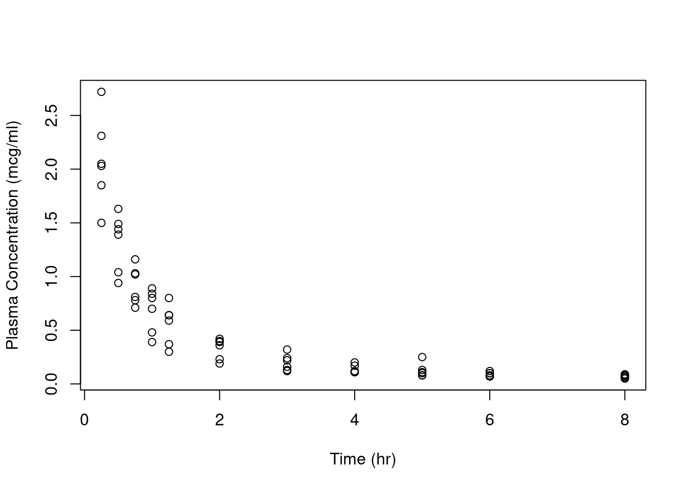
This data does not look linear. We might consider a log transform of the
variable conc for blood concentration, but that doesn’t fix the problem
either. We may prefer a nonlinear model to describe the relationship between
these variables.
We will use instead a linearly combined bi-exponential model. Let \(C\) represent plasma concentration of the drug and \(t\) time. All other variables in the equation below are model parameters we will need to estimate.
\[C_t = C_0 + a_1 e^{-b_1 t} + a_2 e^{-b_2 t}\]
Since we have different subjects \(i\) and measurement “errors” \(\epsilon_{it}\), we instead consider the following statistical model:
\[C_{it} = C_0 + a_1 e^{-b_1 t} + a_2 e^{-b_2 t} + \epsilon_{it}.\]
The R function below encapsulates the relationship between time and concentration.
doubexpfunc <- function(t, C0, a1, a2, b1, b2) {
  C0 + a1 * exp(-b1 * t) + a2 * exp(-b2 * t)
}

curve(doubexpfunc(x, 0.125, 0.75, 1, 1.5, 1.1), from = 0, to = 8.25,
      xlab = "Time (hr)", ylab = "Plasma Concentration (mcg/ml)")
points(conc ~ time, data = Indometh, pch = 20)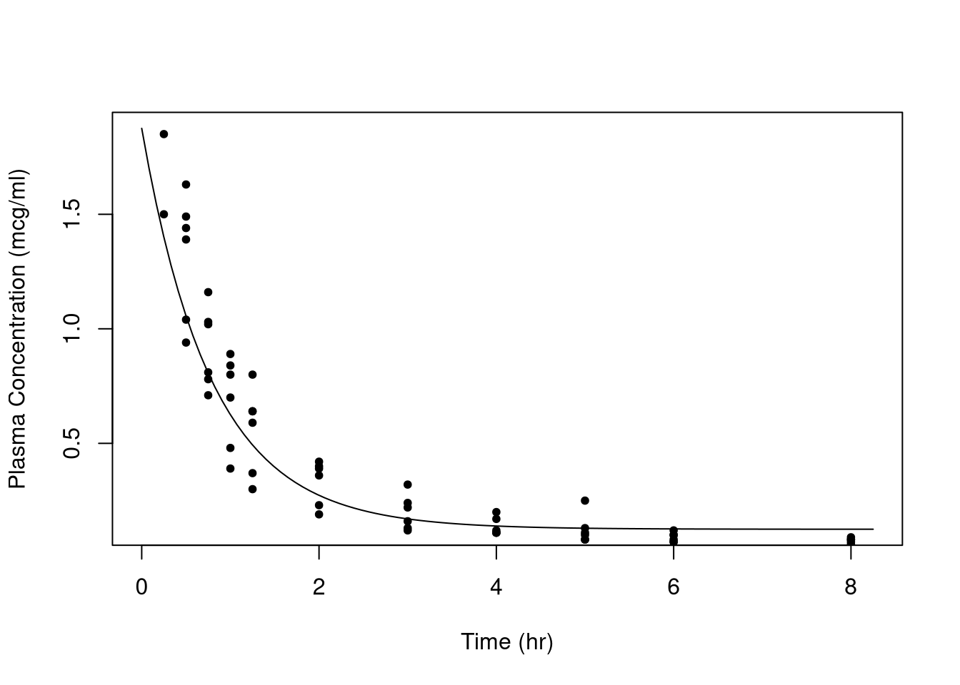
Above is the function with a guess at the parameter values superimposed on the data. Is the guess good? No, but it’s close enough for the numerical techniques.
We actually get an estimated fit using these initial guesses like so:
(fit <- nls(conc ~ doubexpfunc(time, C0, a1, a2, b1, b2), data = Indometh,
        start = c(C0 = 0.125, a1 = 0.75, a2 = 1, b1 = 1.5, b2 = 1.1)))
## Nonlinear regression model
## model: conc ~ doubexpfunc(time, C0, a1, a2, b1, b2)
## data: Indometh
## C0 a1 a2 b1 b2
## 0.07393 2.53684 0.95687 3.01862 0.66572
## residual sum-of-squares: 1.872
##
## Number of iterations to convergence: 9
## Achieved convergence tolerance: 7.851e-06##
## Formula: conc ~ doubexpfunc(time, C0, a1, a2, b1, b2)
##
## Parameters:
## Estimate Std. Error t value Pr(>|t|)
## C0 0.07393 0.06461 1.144 0.2570
## a1 2.53684 0.54544 4.651 1.82e-05 ***
## a2 0.95687 0.74799 1.279 0.2057
## b1 3.01862 1.40640 2.146 0.0358 *
## b2 0.66572 0.46825 1.422 0.1602
## ---
## Signif. codes: 0 '***' 0.001 '**' 0.01 '*' 0.05 '.' 0.1 ' ' 1
##
## Residual standard error: 0.1752 on 61 degrees of freedom
##
## Number of iterations to convergence: 9
## Achieved convergence tolerance: 7.851e-06## [1] "nls"## C0 a1 a2 b1 b2
## 0.07393449 2.53684071 0.95686744 3.01862352 0.66571921A lot of the least-squares theory developed in the linear regression case carry over to nonlinear regression. For example, we can perform inference for model parameters using the \(t\)-test and assess the quality of the model fit with the AIC. Below is a plot of the resulting fit.
fitted_doubexpfunc <- function(fit) {
  C0 <- coef(fit)["C0"]
  a1 <- coef(fit)["a1"]
  a2 <- coef(fit)["a2"]
  b1 <- coef(fit)["b1"]
  b2 <- coef(fit)["b2"]
  function(t) {
    doubexpfunc(t, C0, a1, a2, b1, b2)
  }
}

fit_func <- fitted_doubexpfunc(fit)
curve(fit_func(x), from = 0, to = 8.25, xlab = "Time (hr)",
      ylab = "Plasma Concentration (mcg/ml)")
points(conc ~ time, data = Indometh, pch = 20)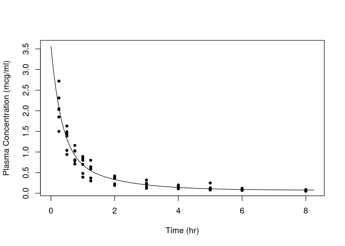
All told the fit looks rather good. (Note that predict() can also be used for
making predictions from the model.)
Be aware that nonlinear models are generally more complicated to estimate than linear models, if only because in addition to asking questions about the statistical quality about the model, practitioners should be sensitive to numerical issues as well. For example, one may need to decide on the maximum number of iterations for the solver, the desirable numerical tolerance, where to pick the starting values, what to do when the gradient matrix is near-singular, and so on. All told there are many more points of failure for nonlinear models that we will not discuss here.