Lecture 10
Multiple Linear Regression
My presentation up to now has been focused on the simple linear model but has suggested the possibility of multiple explanatory variables. In fact regression with multiple variables is technically not much different from simple linear regression. Much of what we’ve said transfers over, though the issues of model selection become more interesting.
Estimation
Estimating a model with multiple explanatory variables is easy; just add those variables into the model.
Let’s for example study the data set mtcars and examine the influence of
variables on the miles per gallon of a vehicle.
##                    mpg cyl disp  hp drat    wt  qsec vs am gear carb
## Mazda RX4         21.0   6  160 110 3.90 2.620 16.46  0  1    4    4
## Mazda RX4 Wag     21.0   6  160 110 3.90 2.875 17.02  0  1    4    4
## Datsun 710        22.8   4  108  93 3.85 2.320 18.61  1  1    4    1
## Hornet 4 Drive    21.4   6  258 110 3.08 3.215 19.44  1  0    3    1
## Hornet Sportabout 18.7   8  360 175 3.15 3.440 17.02  0  0    3    2
## Valiant 18.1 6 225 105 2.76 3.460 20.22 1 0 3 1##
## Call:
## lm(formula = mpg ~ disp + hp, data = mtcars)
##
## Residuals:
## Min 1Q Median 3Q Max
## -4.7945 -2.3036 -0.8246 1.8582 6.9363
##
## Coefficients:
## Estimate Std. Error t value Pr(>|t|)
## (Intercept) 30.735904 1.331566 23.083 < 2e-16 ***
## disp -0.030346 0.007405 -4.098 0.000306 ***
## hp -0.024840 0.013385 -1.856 0.073679 .
## ---
## Signif. codes: 0 '***' 0.001 '**' 0.01 '*' 0.05 '.' 0.1 ' ' 1
##
## Residual standard error: 3.127 on 29 degrees of freedom
## Multiple R-squared: 0.7482, Adjusted R-squared: 0.7309
## F-statistic: 43.09 on 2 and 29 DF, p-value: 2.062e-09##
## ===============================================
## Dependent variable:
## ---------------------------
## mpg
## -----------------------------------------------
## disp -0.030***
## (0.007)
##
## hp -0.025*
## (0.013)
##
## Constant 30.736***
## (1.332)
##
## -----------------------------------------------
## Observations 32
## R2 0.748
## Adjusted R2 0.731
## Residual Std. Error 3.127 (df = 29)
## F Statistic 43.095*** (df = 2; 29)
## ===============================================
## Note: *p<0.1; **p<0.05; ***p<0.01In statistics, a variable that takes the values of either 0 or 1 depending on
whether a condition is true or not is called a dummy variable or indicator
variable. In the mtcars data set, the variables vs and am are indicator
variables tracking the shape of the engine of a car and whether a car has an
automatic transmission, respectively. These variables are already conveniently
encoded as 0/1 variables.
##
## ===============================================
##                         Dependent variable:
##                     ---------------------------
##                                 mpg
## -----------------------------------------------
## disp                          -0.014
##                               (0.009)
##
## hp                           -0.041***
##                               (0.014)
##
## am                            3.796**
##                               (1.424)
##
## Constant                     27.866***
##                               (1.620)
##
## -----------------------------------------------
## Observations                    32
## R2                             0.799
## Adjusted R2                    0.778
## Residual Std. Error       2.842 (df = 28)
## F Statistic           37.149*** (df = 3; 28)
## ===============================================
## Note:               *p<0.1; **p<0.05; ***p<0.01
Oh, look at that! Our original model saved in fit had a statistically
significant coefficient for disp but that’s not the case for fit2. We will
need to look into this. It’s possible that the reason why this occured is
because the original model suffered from omitted variable bias (OMB), where
two potential regressors were correlated with each other but only one of them
had a meaningful effect on the response variable. But perhaps the issue instead
is that the new model suffers from multicollinearity, which means that there
is a strong linear relationship between two variables; in the case of perfect
multicollinearity, where one regressor is exactly a linear combination of
the other variables (that is, we could say that some variables \(z_1, \ldots, z_p\) satisfy \(z_1 = b_1 + b_2 z_2 + \ldots + b_p z_p\) for some coefficients
\(b_1, \ldots, b_p\)), the model cannot be estimated at all (though often software
detects this and simply removes variables until the perfect multicollinearity is
gone). A consequence of multicollinearity is large standard errors in model
coefficients, which makes precise estimation and inference difficult. One can
understand the phenomenon as struggling to distinguish the effects of two
variables that are strongly related to each other. A third possibility is that
one of these variables are irrelevant and increase the standard errors of
the other coefficient estimates in the model. Here either omitted variable bias
or multicollinearity are likely producing these results, and we would need to
decide between them. (I’m inclined to believe the issue is OMB: am was an
omitted variable and disp actually might not belong in the model.)
Suppose we want to account for the cylinders in our model, along with the shape
of the engine. We could include cyl and vs as variables. Additionally, we
could allow for an interaction between the variables by multiplying cyl with
vs. The resulting model is estimated below:
##
## ===============================================
##                         Dependent variable:
##                     ---------------------------
##                                 mpg
## -----------------------------------------------
## disp                          -0.010
##                               (0.011)
##
## hp                           -0.038**
##                               (0.015)
##
## am                            3.867**
##                               (1.651)
##
## cyl                            0.417
##                               (1.050)
##
## vs                            10.903*
##                               (6.058)
##
## cyl:vs                        -1.724
##                               (1.051)
##
## Constant                     22.474***
##                               (6.060)
##
## -----------------------------------------------
## Observations                    32
## R2                             0.830
## Adjusted R2                    0.789
## Residual Std. Error       2.766 (df = 25)
## F Statistic           20.357*** (df = 6; 25)
## ===============================================
## Note:               *p<0.1; **p<0.05; ***p<0.01
You probably have noticed that + in a formula does not mean literal additiona,
and * does not mean literal multiplication. Both operators have been
overloaded in the context of formulas. The effect of * here is to include
terms in the model for both the variables cyl and vs separately and a term
representing the product of these two variables. If we wanted literal
multiplication in the model, we would have to encapsulate that multiplication
with the I() function. The model below is equivalent to fit3.
##
## ===============================================
##                         Dependent variable:
##                     ---------------------------
##                                 mpg
## -----------------------------------------------
## disp                          -0.010
##                               (0.011)
##
## hp                           -0.038**
##                               (0.015)
##
## am                            3.867**
##                               (1.651)
##
## cyl                            0.417
##                               (1.050)
##
## vs                            10.903*
##                               (6.058)
##
## I(cyl * vs)                   -1.724
##                               (1.051)
##
## Constant                     22.474***
##                               (6.060)
##
## -----------------------------------------------
## Observations                    32
## R2                             0.830
## Adjusted R2                    0.789
## Residual Std. Error       2.766 (df = 25)
## F Statistic           20.357*** (df = 6; 25)
## ===============================================
## Note:               *p<0.1; **p<0.05; ***p<0.01
Perhaps we should incorporate cylinders in a different way, though; perhaps
cylinders should be treated as categorical variables. This could allow for
non-linear effects in the number of cylinders. We could force cylinders to be
treated as categorical variables by passing them as factors to the model, like
so (note that if the variable cyl was already a factor variable, as.factor()
would not be needed):
##
## ===============================================
##                         Dependent variable:
##                     ---------------------------
##                                 mpg
## -----------------------------------------------
## disp                          -0.015
##                               (0.011)
##
## hp                           -0.039**
##                               (0.015)
##
## am                            3.334**
##                               (1.364)
##
## as.factor(cyl)6               -3.222*
##                               (1.589)
##
## as.factor(cyl)8               -1.011
##                               (3.033)
##
## Constant                     29.004***
##                               (1.845)
##
## -----------------------------------------------
## Observations                    32
## R2                             0.837
## Adjusted R2                    0.806
## Residual Std. Error       2.653 (df = 26)
## F Statistic           26.790*** (df = 5; 26)
## ===============================================
## Note:               *p<0.1; **p<0.05; ***p<0.01
Linear models handle categorical variables by producing a dummy variable for the possible values of the categorical variable. Specifically, all categories but one get a dummy variable that indicates whether the observation was in that category or not. One category is omitted because otherwise the dummy variables would become collinear with the intercept term; the group that does not get a dummy variable become the baseline group. This is because the coefficients of the other variables are effectively contrasts with the mean of the baseline group. This follows from the interpretation of the coefficients of dummy variables: they are the change in expected value when that variable is true or not. If we did not want a baseline group, we would need to suppress the constant; then all groups in the categorical variable will get a dummy variable.
##
## ===============================================
##                         Dependent variable:
##                     ---------------------------
##                                 mpg
## -----------------------------------------------
## disp                          -0.015
##                               (0.011)
##
## hp                           -0.039**
##                               (0.015)
##
## am                            3.334**
##                               (1.364)
##
## as.factor(cyl)4              29.004***
##                               (1.845)
##
## as.factor(cyl)6              25.782***
##                               (2.542)
##
## as.factor(cyl)8              27.993***
##                               (4.237)
##
## -----------------------------------------------
## Observations                    32
## R2                             0.987
## Adjusted R2                    0.984
## Residual Std. Error       2.653 (df = 26)
## F Statistic           328.109*** (df = 6; 26)
## ===============================================
## Note:               *p<0.1; **p<0.05; ***p<0.01
The coefficients of the factor variables in the new model can be interpreted as the mean MPG for each count of cylinders, without yet accounting for the effects of the other variables in the model.
Inference and Model Selection
All the statistical procedures discussed with simple linear regression apply in the multivariate setting, including the diagnostic tools, but some issues should be updated.
First, regarding the \(F\)-test. The \(F\)-test as described before still works as marketed, but we can make additional \(F\) tests to help decide between models. For instance, we could decide between
\[H_0: \beta_{k^*} = \beta_{k^* + 1} = \cdots = \beta_k = 0\]
and
\[H_A: H_0 \text{ is false}\]
for some \(k^* \geq 1\). In other words, we can test whether a collection of new regressors have predictive power when added to a smaller linear model.
We may, for example, want to test whether any of the coefficients in fit4 are
non-zero, comparing against the model contained in fit. To perform this test,
we should use the anova() function (another function that can perform
anova()) like so:
## Analysis of Variance Table
##
## Model 1: mpg ~ disp + hp
## Model 2: mpg ~ disp + hp + am + as.factor(cyl)
##   Res.Df    RSS Df Sum of Sq      F   Pr(>F)
## 1     29 283.49
## 2     26 183.04  3    100.45 4.7564 0.008961 **
## ---
## Signif. codes:  0 '***' 0.001 '**' 0.01 '*' 0.05 '.' 0.1 ' ' 1
The results of the above test suggest that some of the coefficients in the model
fit4 are not zero; one should necessarily conclude that fit4 is a better
model than fit, since fit is missing important variables.
Next, let’s consider the issue of confidence intervals. vcov() still works.
##                  (Intercept)          disp            hp           am
## (Intercept)      3.405382437 -0.0127499444 -0.0067209058 -1.195577901
## disp            -0.012749944  0.0001120357 -0.0000423764  0.006150034
## hp              -0.006720906 -0.0000423764  0.0002208071 -0.009721922
## am              -1.195577901  0.0061500337 -0.0097219220  1.859508755
## as.factor(cyl)6  0.266125814 -0.0052414970 -0.0083459097  0.460108720
## as.factor(cyl)8  2.673529289 -0.0188226829 -0.0231231395  0.792321864
##                 as.factor(cyl)6 as.factor(cyl)8
## (Intercept)         0.266125814      2.67352929
## disp               -0.005241497     -0.01882268
## hp                 -0.008345910     -0.02312314
## am                  0.460108720      0.79232186
## as.factor(cyl)6     2.523821471      3.26500050
## as.factor(cyl)8 3.265000500 9.20011728## (Intercept) disp hp am
## (Intercept) 1.00000000 -0.6527504 -0.2450972 -0.4751118
## disp -0.65275043 1.0000000 -0.2694259 0.4260889
## hp -0.24509720 -0.2694259 1.0000000 -0.4797848
## am -0.47511180 0.4260889 -0.4797848 1.0000000
## as.factor(cyl)6 0.09077677 -0.3117079 -0.3535394 0.2123890
## as.factor(cyl)8 0.47764509 -0.5862821 -0.5130310 0.1915604
## as.factor(cyl)6 as.factor(cyl)8
## (Intercept) 0.09077677 0.4776451
## disp -0.31170793 -0.5862821
## hp -0.35353943 -0.5130310
## am 0.21238901 0.1915604
## as.factor(cyl)6 1.00000000 0.6775748
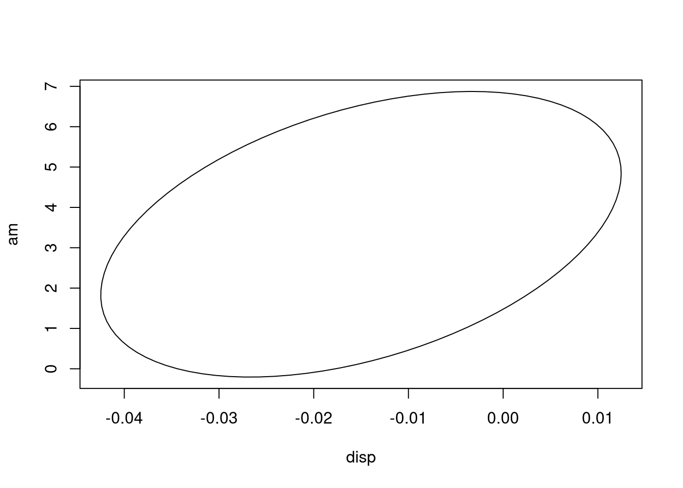
## as.factor(cyl)8 0.67757481 1.0000000Again, the confidence region is an elliptical space, but this time in \(k + 1\)
dimensional space, rather than two-dimensional space. Attempting to visualize
high-dimensional space directly is known to induce madness, so we may be better
off looking at pairs of relationships between coefficients. We can do so by
telling the ellipse() function we saw earlier which variables we wish to
visualize.
library(ellipse)
plot_conf_ellipse <- function(..., col = 1, add = FALSE) {
  if (add) {
    pfunc = lines
  } else {
    pfunc = plot
  }
  pfunc(ellipse(...), type = "l", col = col)
}

plot_conf_ellipse(fit4, which = c("(Intercept)", "disp"))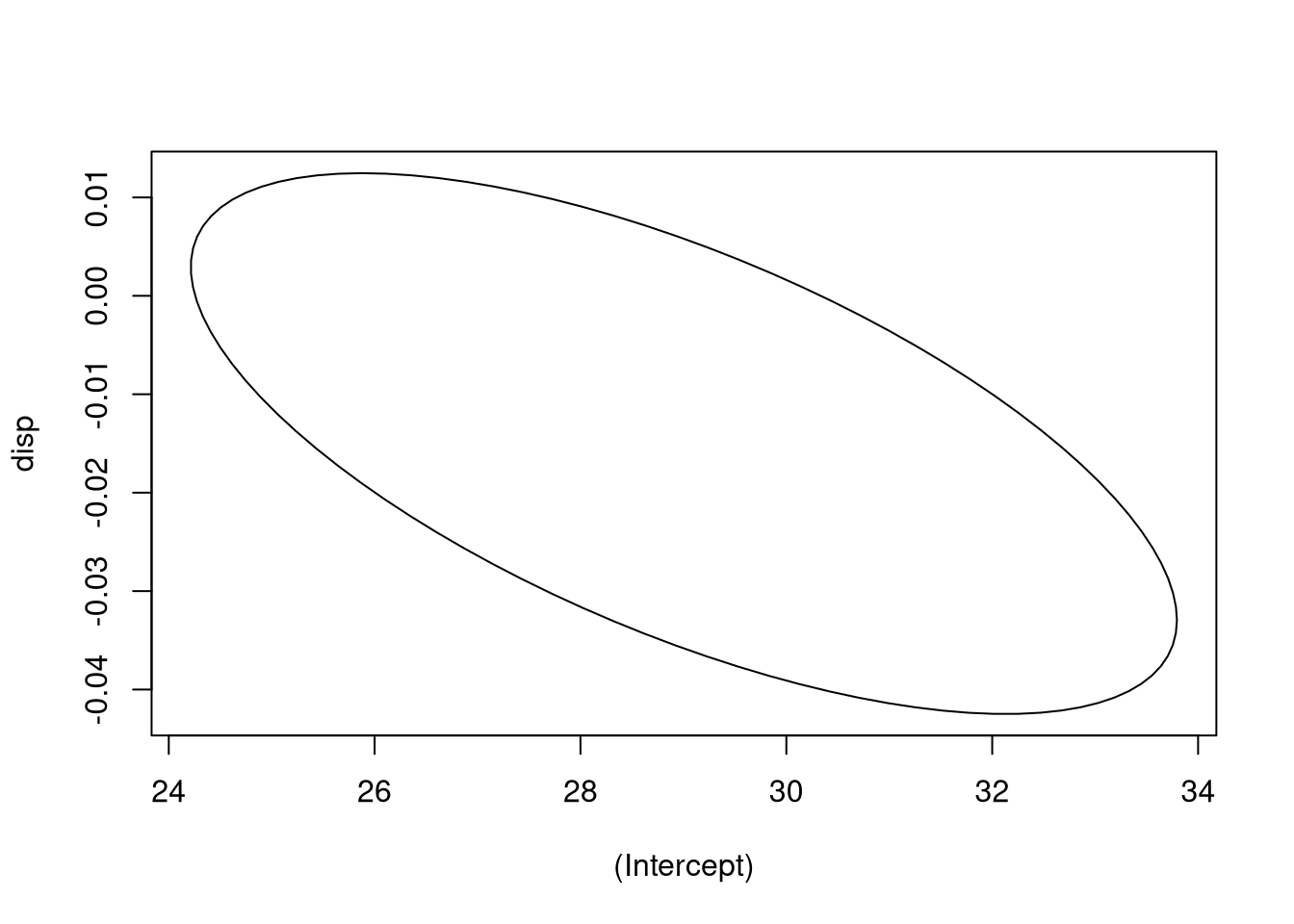
Suppose we wish to predict values from our model, maybe also get point-wise
confidence intervals or prediction intervals. We will need to use the
predict() function as we did before. For what it’s worth, predict() works
exactly the same; it needs to be fed a data.frame containing the new values of
the model’s regressors, in a format imitating the original data. (You don’t need
to manually create automatically generated dummy variables, for example, or
insert columns for interaction variables.) Visualizing the predictions, though,
will be more difficult due to the multivariate setting. (In general, if you want
to learn more about multivariate visualization techniques, consider taking a
class dedicated to visualization.)
While predict() has not changed, my function predict_func() should be
adapted to the new setting.
predict_func_multivar <- function(fit) {
  function(..., interval = "none", level = 0.95) {
    dat <- data.frame(...)
    predict(fit, dat, interval = interval, level = level)
  }
}

mtcar_pf <- predict_func_multivar(fit2)
mtcar_pf(disp = c(160, 150), hp = c(110, 80), am = c(0, 1))
## 1 2
## 21.06192 26.24082## fit lwr upr
## 1 21.06192 19.06074 23.06309
## 2 26.24082 24.09598 28.38566Now let’s consider criteria for deciding between models. This is new to the multivariate context; in simple linear regression there’s no interesting model selection discussion to be had. But for multivariate models, we have to decide which coefficients to include or exclude and in what functional form they should appear. At first one may think that one should check the statistical significance of model coefficients and \(F\)-tests and use those results to decide what model is most appropriate for the data. This approach is mistaken. First, it’s path-dependent; if we choose a different sequence of models to check we may end up with different end results for coefficients. It also doesn’t inform us well regarding how we should handle changing test results as we insert and delete coefficients; coefficients that once weren’t significant could become significant after inserting or deleting another regressor, or vice versa. Secondly, this is multiple hypothesis testing; the hypothesis tests start to lose their statistical guarantees as we test repeatedly.
Okay, how about checking the value of \(R^2\) or adjusted \(R^2\)? While we should be sensitive to the value of \(R^2\), we must use it with great caution. Perfectly valid and acceptable statistical models have low \(R^2\) models, and bad models can have high \(R^2\) values. We have two competing concerns: underfitting and overfitting. Underfitting means our model has little predictive power and could be improved. Models that have been overfitted, though, have excellent predictive power in the observed sample, but say little about the general population and lose their predictive power when we feed them new, out-of-sample data. Attempting to maximize \(R^2\) can easily lead to overfitting, and thus should be avoided. However, a low \(R^2\) might indicate underfitting.
We need more tools for model selection. One useful tool is the Akaike
information criterion (AIC), a statistic intended to estimate the
out-of-sample predictive power of a model. We can obtain the AIC for a
particular model using the AIC() function.
## [1] 168.6186There is no universal interpretation of the AIC itself (at least not one that’s not heavily theoretical). The AIC should not be considered in isolation, though; instead, we compare the AIC statistics of competing candidate models, selecting the model that minimizes the AIC. We can even get a reasonable interpretation of AICs when comparing two. If we have \(AIC_1\) and \(AIC_2\) for two different models, then we can interpret the quantity
\[\operatorname{exp}\left((AIC_1 - AIC_2)/2\right)\]
as how many more times the model with \(AIC_2\) is likely to be true than the model with \(AIC_1\). The function below performs this kind of analysis:
## [1] 54.58818That said, we are generally interested in just finding the model that minimizes the AIC among a class of similar models. The function below can find such a model, when given a list of models.
min_aic_model <- function(...) {
  models <- list(...)
  aic_list <- sapply(models, AIC)
  best_model <- models[[which.min(aic_list)]]
  best_model
}

best_fit <- min_aic_model(fit, fit2, fit3, fit4)
stargazer(best_fit, type = "text")
##
## ===============================================
## Dependent variable:
## ---------------------------
## mpg
## -----------------------------------------------
## disp -0.015
## (0.011)
##
## hp -0.039**
## (0.015)
##
## am 3.334**
## (1.364)
##
## as.factor(cyl)6 -3.222*
## (1.589)
##
## as.factor(cyl)8 -1.011
## (3.033)
##
## Constant 29.004***
## (1.845)
##
## -----------------------------------------------
## Observations 32
## R2 0.837
## Adjusted R2 0.806
## Residual Std. Error 2.653 (df = 26)
## F Statistic 26.790*** (df = 5; 26)
## ===============================================
## Note: *p<0.1; **p<0.05; ***p<0.01## [1] 0.01831898 0.25140981 0.18120055 1.00000000It seems that the fourth model seems to best describe the data. That said, some of the coefficients in the model are not statistically different from zero. That’s okay; sometimes a good model needs these regressors. However, be aware that model selection via AIC is an asymptotic method; the sample size needs to be large for the AIC to work well.
You may be tempted to write a script that tries just about every combination of parameters and functional forms in a linear model, finds the one with the smallest AIC, and returns it; it’s an automatic statistician that would put you out of a job if your employers were aware of it. Resist the temptation! The AIC is a tool to help pick models, but is not a substitute for human domain knowledge. Left to its own devices, the AIC could select models that don’t have the best predictive power because they make no sense, and any subject matter expert would say so. The most important model selection tool is human knowledge of the problem. Lean heavily on it! Consider only models that make sense. Consult experts in the subject before building models.
Polynomial Regression
Let’s back up and return to the univarate context, where we have one explanatory variable and one response variable. Why should we consider models only of the form \(y = a + bx\)? Why not quadratic models, \(y = a + bx + cx^2\)? Or higher-order polynomials, \(y = \beta_0 + \beta_1 x + \beta_2 x^2 + \cdots + \beta_k x^k\)? Well, we can in fact consider such models, and we call the topic polynomial regression. These are regression models of the form:
\[y_i = \beta_0 + \beta_1 x_i + \beta_2 x_i^2 + \cdots + \beta_k x_i^k + \epsilon_i.\]
We can view these models as multivariate models; we just add the variables \(x\), \(x^2\), \(x^3\), and so on to our model. These variabes are not linearly related to each other, so we can generally estimate such models.
Let’s demonstrate by simulating a data set that takes a cubic form on the interval \([-1, 1]\). This will be a cubic function plus some noise.
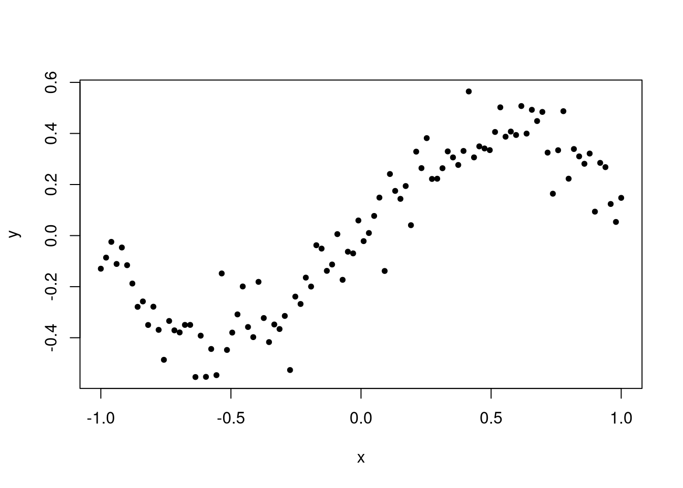
Clearly a model that is just a line is not appropriate for this data set; diagnostic plots would reveal this.
##
## Call:
## lm(formula = y ~ x)
##
## Residuals:
##      Min       1Q   Median       3Q      Max
## -0.41483 -0.13292 -0.00562  0.13003  0.38619
##
## Coefficients:
##             Estimate Std. Error t value Pr(>|t|)
## (Intercept) 0.007171   0.018084   0.397    0.693
## x           0.435494   0.031010  14.043   <2e-16 ***
## ---
## Signif. codes:  0 '***' 0.001 '**' 0.01 '*' 0.05 '.' 0.1 ' ' 1
##
## Residual standard error: 0.1808 on 98 degrees of freedom
## Multiple R-squared:  0.668,  Adjusted R-squared:  0.6647
## F-statistic: 197.2 on 1 and 98 DF,  p-value: < 2.2e-16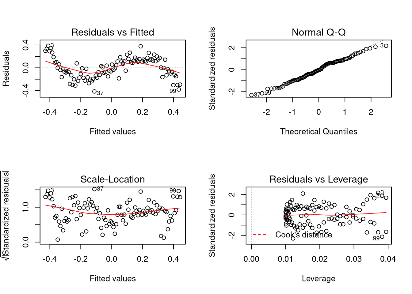
## Warning in par(old_par): graphical parameter "cin" cannot be set## Warning in par(old_par): graphical parameter "cra" cannot be set## Warning in par(old_par): graphical parameter "csi" cannot be set## Warning in par(old_par): graphical parameter "cxy" cannot be set## Warning in par(old_par): graphical parameter "din" cannot be set## Warning in par(old_par): graphical parameter "page" cannot be set
The problem is that the data should be about evenly distributed around the line, but instead we see data being more likely to be above the line at the start of the window, below in the first half, above in the second half, and below at the very end. This indicates an inappropriate functional form, and we should rectify the issue.
Notice the estimated values? We see that the estimated coefficient for the intercept term is close to zero, and for the linear term close to 0.4. We know that the value of these coefficients in the true model are zero and one, respectively, but these parameters are not even close to the true values.
plot(c(0, fit$coefficients[[1]]), c(1, fit$coefficients[[2]]), pch = 20,
     xlim = c(-0.1, 0.1), ylim = c(0.1, 1.1), xlab = expression(beta[0]),
     ylab = expression(beta[1]))
plot_conf_ellipse(fit, add = TRUE)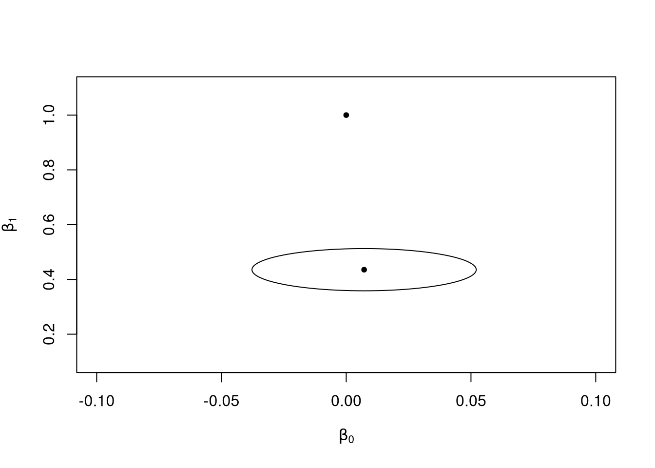
When the model is misspecified this way, the eventual “best” values for \(\beta_0\) and \(\beta_1\) are 0 and 0.4 rather than the true values of 0 and 1. That is, if \(f(x) = x - x^3\) and \(\hat{f}(x; \beta_0, \beta_1) = \beta_0 + \beta_1 x\), the regression model will estimate the values \(\beta_0\) and \(\beta_1\) that minimize
\[S(\beta_0, \beta_1) = \int_{-1}^{1} (f(x) - \hat{f}(x; \beta_0, \beta_1))^2 dx = \int_{-1}^{1} (x - x^3 - \beta_0 - \beta_1 x)^2 dx.\]
Perhaps if we were to include a quadratic term? We can do so using the I()
function (we cannot call ^ directly in a formula; this has special meaning in
formulas other than exponentiation).
fit2 <- lm(y ~ x + I(x^2))

predict_func <- function(fit) {
  response <- names(fit$model)[[1]]
  explanatory <- names(fit$model)[[2]]
  function(x, ...) {
    dat <- data.frame(x)
    names(dat) <- explanatory
    predict(fit, dat, ...)
  }
}

summary(fit2)
##
## Call:
## lm(formula = y ~ x + I(x^2))
##
## Residuals:
## Min 1Q Median 3Q Max
## -0.40738 -0.13768 -0.00702 0.13137 0.38166
##
## Coefficients:
## Estimate Std. Error t value Pr(>|t|)
## (Intercept) -0.00237 0.02724 -0.087 0.931
## x 0.43549 0.03113 13.988 <2e-16 ***
## I(x^2) 0.02806 0.05970 0.470 0.639
## ---
## Signif. codes: 0 '***' 0.001 '**' 0.01 '*' 0.05 '.' 0.1 ' ' 1
##
## Residual standard error: 0.1816 on 97 degrees of freedom
## Multiple R-squared: 0.6688, Adjusted R-squared: 0.662
## F-statistic: 97.94 on 2 and 97 DF, p-value: < 2.2e-16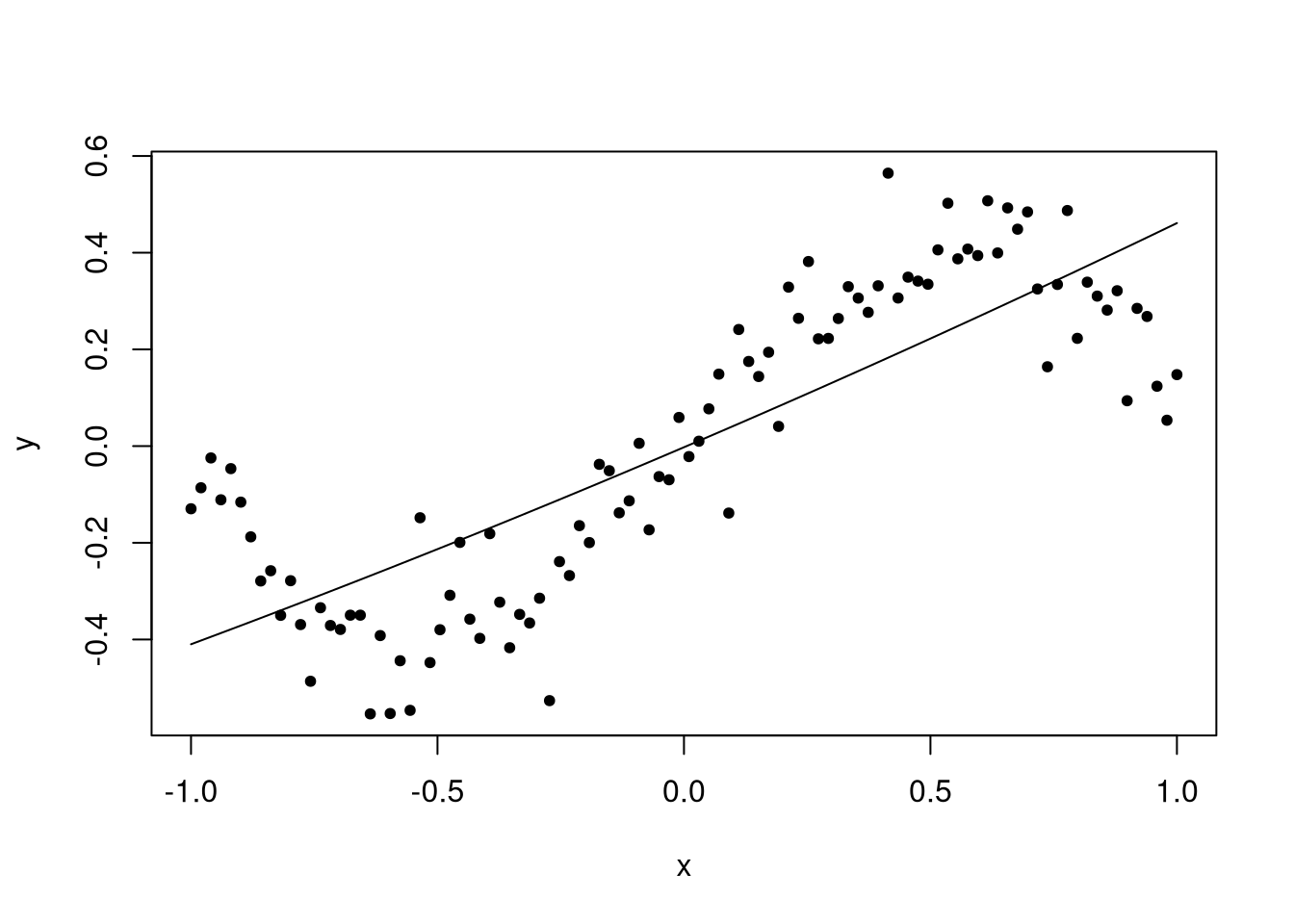
Unfortunately the quadratic model is not a big improvement. But did you notice that the resulting predicted line has a slight bend? There was an effort to fit the line but it didn’t quite work. But of course it didn’t; the model is incorrect, and the true value of the quadratic coefficient is zero. What we should do is insert a cubic term.
##
## Call:
## lm(formula = y ~ x + I(x^2) + I(x^3))
##
## Residuals:
##       Min        1Q    Median        3Q       Max
## -0.261069 -0.039120 -0.001413  0.051662  0.253088
##
## Coefficients:
##             Estimate Std. Error t value Pr(>|t|)
## (Intercept) -0.00237    0.01356  -0.175    0.862
## x            1.04617    0.03875  26.995   <2e-16 ***
## I(x^2)       0.02806    0.02971   0.944    0.347
## I(x^3)      -0.99777    0.05804 -17.192   <2e-16 ***
## ---
## Signif. codes:  0 '***' 0.001 '**' 0.01 '*' 0.05 '.' 0.1 ' ' 1
##
## Residual standard error: 0.09037 on 96 degrees of freedom
## Multiple R-squared:  0.9188, Adjusted R-squared:  0.9163
## F-statistic: 362.1 on 3 and 96 DF,  p-value: < 2.2e-16
Now our model has a good fit to the data, and the estimated coefficients are close to the truth.
Should we have included the quadratic term even when we believed it might be wrong? The answer is yes. In general we won’t know what the true model is so we must include all polynomial orders up to the highest order \(k\).
Okay, but by that same reasoning we don’t know that there isn’t a fourth-order term, or even higher, in our polynomial. Should we start including those terms too? Let’s see what happens when we do.
##
## Call:
## lm(formula = y ~ x + I(x^2) + I(x^3) + I(x^4))
##
## Residuals:
##       Min        1Q    Median        3Q       Max
## -0.262997 -0.039840 -0.002202  0.053533  0.258240
##
## Coefficients:
##              Estimate Std. Error t value Pr(>|t|)
## (Intercept)  0.003425   0.017008   0.201    0.841
## x            1.046172   0.038892  26.900   <2e-16 ***
## I(x^2)      -0.028775   0.104447  -0.276    0.784
## I(x^3)      -0.997775   0.058243 -17.131   <2e-16 ***
## I(x^4)       0.065012   0.114508   0.568    0.572
## ---
## Signif. codes:  0 '***' 0.001 '**' 0.01 '*' 0.05 '.' 0.1 ' ' 1
##
## Residual standard error: 0.09069 on 95 degrees of freedom
## Multiple R-squared:  0.9191, Adjusted R-squared:  0.9157
## F-statistic: 269.7 on 4 and 95 DF,  p-value: < 2.2e-16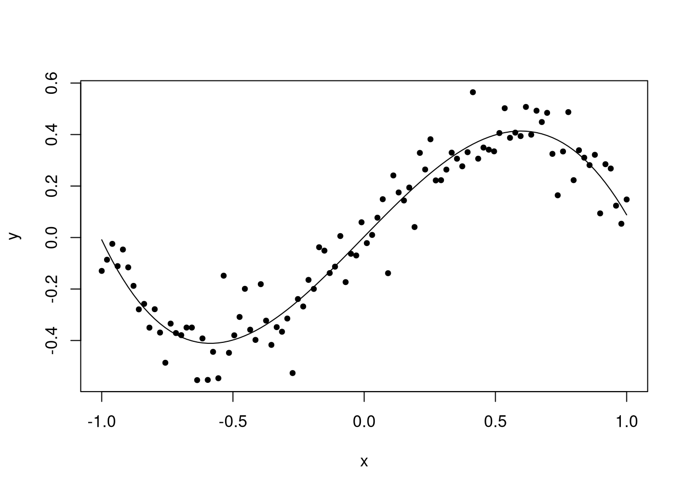
fit10 <- lm(y ~ x + I(x^2) + I(x^3) + I(x^4) + I(x^5) + I(x^6) + I(x^7) +
                I(x^8) + I(x^9) + I(x^10))
summary(fit10)
##
## Call:
## lm(formula = y ~ x + I(x^2) + I(x^3) + I(x^4) + I(x^5) + I(x^6) +
## I(x^7) + I(x^8) + I(x^9) + I(x^10))
##
## Residuals:
## Min 1Q Median 3Q Max
## -0.252290 -0.045165 -0.002792 0.059457 0.239424
##
## Coefficients:
## Estimate Std. Error t value Pr(>|t|)
## (Intercept) 0.009697 0.024615 0.394 0.695
## x 1.126094 0.140917 7.991 4.53e-12 ***
## I(x^2) -0.539507 0.704245 -0.766 0.446
## I(x^3) -2.377790 1.572412 -1.512 0.134
## I(x^4) 5.426529 5.164854 1.051 0.296
## I(x^5) 6.071780 5.549105 1.094 0.277
## I(x^6) -17.991760 14.372753 -1.252 0.214
## I(x^7) -9.444141 7.561495 -1.249 0.215
## I(x^8) 23.460682 16.774469 1.399 0.165
## I(x^9) 4.736288 3.484055 1.359 0.177
## I(x^10) -10.385099 6.924511 -1.500 0.137
## ---
## Signif. codes: 0 '***' 0.001 '**' 0.01 '*' 0.05 '.' 0.1 ' ' 1
##
## Residual standard error: 0.09083 on 89 degrees of freedom
## Multiple R-squared: 0.9239, Adjusted R-squared: 0.9154
## F-statistic: 108.1 on 10 and 89 DF, p-value: < 2.2e-16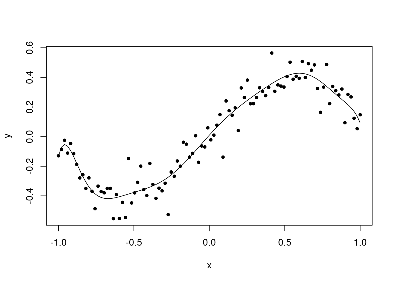
The quality of the fit is degrading. In my opinion, the last function is clearly not the same as the true function. Below is a plot containing all three functions, with the true function shown as a thick black line.
plot(x, y, pch = 20)
lines(x, x - x^3, lwd = 4)
fit1_func <- predict_func(fit)
lines(x, fit1_func(x), col = "blue", lwd = 2)
lines(x, fit2_func(x), col = "cyan", lwd = 2)
lines(x, fit3_func(x), col = "red", lwd = 2)
lines(x, fit4_func(x), col = "green", lwd = 2)
lines(x, fit10_func(x), col = "purple", lwd = 2)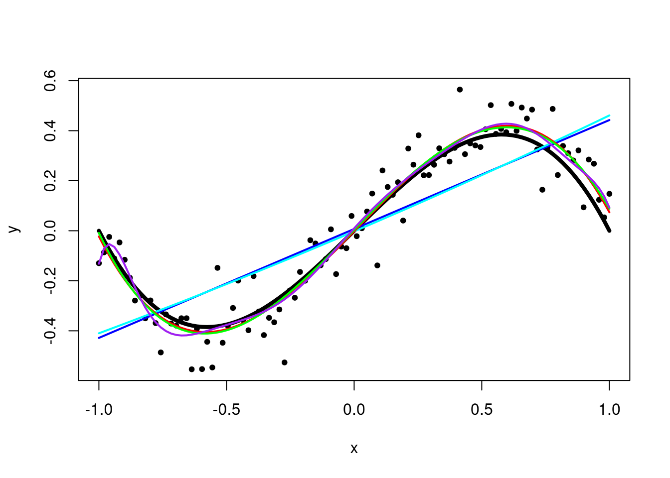
Eventually, if we were to keep adding higher-order terms to the polynomial, we would have an exact fit to the data, where \(\hat{y}_i = y_i\). This is not good since the resulting model would be a monstrosity far from the truth and with no predictive power at all. Thus, when fitting polynomials to data, we want exactly as many polynomial terms as we need and not one more.
That said, what if the true function is not a polynomial? I have exciting news: polynomial regression can fit non-polynomial functions on compact (finite) intervals! The reasons are beyond the scope of this course (go learn more analysis and linear algebra), but any continuous, smooth function can be approximated well by polynomials on compact intervals. Your job, as statistician, is to decide how many polynomial terms you need. Too few and you have a bad fit for the true function; too many and you risk overfitting. But tools such as the AIC can be used to select the proper order of polynomial regression, too.
Here’s what the AIC has to say about the models considered here:
## [1] -54.26317 -52.49059 -191.07099 -189.40972 -183.61339The AIC was minimized for model 3, the third-order polynomial and the correct model order. This of course is not the end of polynomial order selection, but a good first step.