Lecture 8
Linear Regression Models
A linear regression model is a statistical model of the form:
\[y_i = \beta_0 + \beta_1 x_{1i} + \cdots + \beta_k x_{ki} + \epsilon_i.\]
The term \(y_i\) is the response variable or dependent variable, while the variables \(x_{1i}, \ldots, x_{ki}\) are called explanatory variables, independent variables, or regressors. The terms \(\beta_0, \beta_1, \ldots, \beta_k\) are called the coefficients of the model, and \(\epsilon_i\) is the error or residual term. The term \(\beta_0\) is often called the intercept of the model since it’s the predicted value of \(y_i\) when all the explanatory variables are zero.
Simple linear regression refers to a linear regression model with only one explanatory variable:
\[y_i = \beta_0 + \beta_1 x_i + \epsilon_i.\]
This model corresponds to the one-dimensional lines all math students studied in basic algebra, and it’s easily visualized. Additionally, when estimating the model via least-squares estimation, it’s easy and intuitive to write the answer. (Actually the least-squares solution for the full model isn’t hard to write either after one learns some linear algebra, but matrices may scare novice statistics students.) However, the model is generally too simple and real-world applications generally include more than one regressor.
Generally statisticians treat the term \(\epsilon_i\) as the only source of randomness in linear regression models; regressors may or may not be random. Thus most assumption concern the behavior of \(\epsilon_i\), and include assuming that \(E[\epsilon_i] = 0\) and \(\text{Var}(\epsilon_i) = \sigma^2\). We may say more about the errors, such as that the errors are i.i.d. and maybe Normally distributed.
Estimating Simple Linear Regression Models
The models listed above are population models. Our objective is to estimate the parameters of these models. Let \(\hat{\beta}_0\) and \(\hat{\beta}_1\) denote estimates of \(\beta_0\) and \(\beta_1\), respectively. The predicted value of \(y\) given an input \(x\) is:
\[\hat{y} = \hat{\beta}_0 + \hat{\beta}_1 x.\]
We call \(\hat{\epsilon}_i = y_i - \hat{y}_i\) the estimated residual of the model. The question now is how one should estimate the coefficients of the model. The most popular approach is least-squares minimization, where \(\hat{\beta}_0\) and \(\hat{\beta}_1\) are picked such that the sum of square errors:
\[SSE(\hat{\beta}_0, \hat{\beta}_1) = \sum_{i = 1}^N (y_i - \hat{y}_i)^2\]
is minimized. Suppose \(r\) is the sample correlation, \(s_x\) is the sample standard devitation of the explanatory variable, \(s_y\) the sample standard deviation of the response variable, \(\bar{x}\) the sample mean of the explanatory variable, and \(\bar{y}\) the sample mean of the response variable. Then we have a simple solution for the estimates of the coefficients of the least-squares line:
\[\hat{\beta}_1 = r \frac{s_y}{s_x}\]
\[\hat{\beta}_0 = \bar{y} - \hat{\beta}_1 \bar{x}.\]
Practitioners also often wish to estimate the variance of the residuals, \(\sigma^2\), and do so using \(\hat{\sigma}^2 = \frac{1}{n - 2} SSE(\hat{\beta}_1, \hat{\beta}_2)\). The term \(n - 2\) is the degrees of freedom of the simple linear regression model.
When estimating using least squares, the predicted value \(\hat{y}\) can be interpreted as the expected value of the response variable \(y\) given the value of the explanatory variable \(x\). In fact, the predicted value of \(y\) at the mean of the explanatory variables \(\bar{x}\) is \(\bar{y}\). Regression models, however, don’t have to be estimated using the least-squares principle; for example, we could adopt the least absolute deviation principle, and the interpretation of \(\hat{y}\) would change if we did so. Additionally, the coefficients of the model get interpretations; we say that if we increase an input explanatory variable \(x\) by one unit, then we expect \(y\) to be \(\beta_1\) units higher. (The intercept term is generally less interesting in regression models, but its interpretation is clear; it’s the expected value of \(y\) when \(x = 0\).) It’s because of interpretations like these that we may rescale the data, replacing \(x_i\) with \(\frac{x_i - \bar{x}}{s_x}\) and \(y_i\) with \(\frac{y_i - \bar{y}}{s_y}\). Then we would interpret \(\beta_1\) as being how many standard deviations \(y\) changes by when we change \(x\) by one standard deviation. This is a more universally interpretable model.
Linear models are in fact quite expressive; many interesting models can be written as linear models. For instance, consider the model:
\[y_i = \gamma_0 \gamma_1^{x_i} \eta_i.\]
In this model, \(\eta_i\) is the multiplicative residual, and is assumed to be non-negative with mean 1. If we take the natural log of both sides of this equation, we obtain the mode:
\[\ln (y_i) = \ln(\gamma_0) + \ln(\gamma_1) x_i + \ln(\eta_i).\]
This is in fact the linear model we’ve already been considering, but one for \(\ln (y_i)\) rather than \(y_i\) directly. This is known as a log transformation, a useful and popular trick. The interpretations of the coefficients change, though: a unit increase in the exogenous variable causes us to expect a \(\beta_1 \%\) change in \(y_i\). There’s also the model:
\[y_i = \beta_0 + \beta_1 \ln (x_i) + \epsilon_i.\]
In this model a 1% change in the regressor leads to an expected increase of \(\beta_1\) of the response. There’s also the model:
\[\ln(y_i) = \beta_0 + \beta_1 \ln(x_i) + \epsilon_i.\]
Here, a 1% increase in \(x_i\) would cause us to expect a \(\beta_1 \%\) increase in \(y_i\). These interpretations matter, and are a part of model building.
In R, linear models are estimated using the function lm(). If x is the
explanatory variable and y the response variable and both are in a data set
d, we estimate the model using lm(y ~ x, data = d). Generally we save the
results of the fit for later use.
Let’s estimate a linear regression model for the sepal length of iris flowers using the sepal width. We can do so with the following:
##
## Call:
## lm(formula = Sepal.Length ~ Sepal.Width, data = iris)
##
## Coefficients:
## (Intercept)  Sepal.Width
##      6.5262      -0.2234
We don’t need to explicitly tell R to include an intercept term; lm()
automatically includes one. In general you should include intercept terms in
your regression models even if the theoretical model you’re estimating does not
have an intercept term, since doing so helps ensure the residuals of the model
have mean zero. However, if you really want to exclude the intercept term (and
thus be fitting the model \(y_i = \beta x_i + \epsilon_i\)), you can suppress
intercept term estimation like so:
##
## Call:
## lm(formula = Sepal.Length ~ Sepal.Width - 1, data = iris)
##
## Coefficients:
## Sepal.Width
##       1.869
R will print out a basic summary of a lm() fit when the fit object (an object
of class lm) is printed. We can see more information using summary().
##
## Call:
## lm(formula = Sepal.Length ~ Sepal.Width, data = iris)
##
## Residuals:
##     Min      1Q  Median      3Q     Max
## -1.5561 -0.6333 -0.1120  0.5579  2.2226
##
## Coefficients:
##             Estimate Std. Error t value Pr(>|t|)
## (Intercept)   6.5262     0.4789   13.63   <2e-16 ***
## Sepal.Width  -0.2234     0.1551   -1.44    0.152
## ---
## Signif. codes:  0 '***' 0.001 '**' 0.01 '*' 0.05 '.' 0.1 ' ' 1
##
## Residual standard error: 0.8251 on 148 degrees of freedom
## Multiple R-squared:  0.01382,    Adjusted R-squared:  0.007159
## F-statistic: 2.074 on 1 and 148 DF,  p-value: 0.1519
We will discuss later the meaning of this information. That said, while this information is nice, it’s not… pretty. There is a package called stargazer, though, that is meant for making nice presentations of regression results.
##
## Please cite as:
## Hlavac, Marek (2018). stargazer: Well-Formatted Regression and Summary Statistics Tables.## R package version 5.2.2. https://CRAN.R-project.org/package=stargazer##
## ===============================================
## Dependent variable:
## ---------------------------
## Sepal.Length
## -----------------------------------------------
## Sepal.Width -0.223
## (0.155)
##
## Constant 6.526***
## (0.479)
##
## -----------------------------------------------
## Observations 150
## R2 0.014
## Adjusted R2 0.007
## Residual Std. Error 0.825 (df = 148)
## F Statistic 2.074 (df = 1; 148)
## ===============================================
## Note: *p<0.1; **p<0.05; ***p<0.01Actually, stargazer() can print out these regression tables in other formats,
particularly LaTeX and HTML. This makes inserting these tables into other
documents (specifically, papers) easier. (If you want to put your table into a
word processor such as Microsoft Word, try HTML format, and save in an HTML
document; the text processor may be able to convert the HTML table into
something it understands. Or you could just man up and learn LaTeX; it looks
better anyway.)
##
## % Table created by stargazer v.5.2.2 by Marek Hlavac, Harvard University. E-mail: hlavac at fas.harvard.edu
## % Date and time: Sun, Feb 16, 2020 - 12:30:50 PM
## \begin{table}[!htbp] \centering
##   \caption{}
##   \label{}
## \begin{tabular}{@{\extracolsep{5pt}}lc}
## \\[-1.8ex]\hline
## \hline \\[-1.8ex]
##  & \multicolumn{1}{c}{\textit{Dependent variable:}} \\
## \cline{2-2}
## \\[-1.8ex] & Sepal.Length \\
## \hline \\[-1.8ex]
##  Sepal.Width & $-$0.223 \\
##   & (0.155) \\
##   & \\
##  Constant & 6.526$^{***}$ \\
##   & (0.479) \\
##   & \\
## \hline \\[-1.8ex]
## Observations & 150 \\
## R$^{2}$ & 0.014 \\
## Adjusted R$^{2}$ & 0.007 \\
## Residual Std. Error & 0.825 (df = 148) \\
## F Statistic & 2.074 (df = 1; 148) \\
## \hline
## \hline \\[-1.8ex]
## \textit{Note:}  & \multicolumn{1}{r}{$^{*}$p$<$0.1; $^{**}$p$<$0.05; $^{***}$p$<$0.01} \\
## \end{tabular}
## \end{table}##
## <table style="text-align:center"><tr><td colspan="2" style="border-bottom: 1px solid black"></td></tr><tr><td style="text-align:left"></td><td><em>Dependent variable:</em></td></tr>
## <tr><td></td><td colspan="1" style="border-bottom: 1px solid black"></td></tr>
## <tr><td style="text-align:left"></td><td>Sepal.Length</td></tr>
## <tr><td colspan="2" style="border-bottom: 1px solid black"></td></tr><tr><td style="text-align:left">Sepal.Width</td><td>-0.223</td></tr>
## <tr><td style="text-align:left"></td><td>(0.155)</td></tr>
## <tr><td style="text-align:left"></td><td></td></tr>
## <tr><td style="text-align:left">Constant</td><td>6.526<sup>***</sup></td></tr>
## <tr><td style="text-align:left"></td><td>(0.479)</td></tr>
## <tr><td style="text-align:left"></td><td></td></tr>
## <tr><td colspan="2" style="border-bottom: 1px solid black"></td></tr><tr><td style="text-align:left">Observations</td><td>150</td></tr>
## <tr><td style="text-align:left">R<sup>2</sup></td><td>0.014</td></tr>
## <tr><td style="text-align:left">Adjusted R<sup>2</sup></td><td>0.007</td></tr>
## <tr><td style="text-align:left">Residual Std. Error</td><td>0.825 (df = 148)</td></tr>
## <tr><td style="text-align:left">F Statistic</td><td>2.074 (df = 1; 148)</td></tr>
## <tr><td colspan="2" style="border-bottom: 1px solid black"></td></tr><tr><td style="text-align:left"><em>Note:</em></td><td style="text-align:right"><sup>*</sup>p<0.1; <sup>**</sup>p<0.05; <sup>***</sup>p<0.01</td></tr>
## </table>There’s a lot of stargazer() parameters you can modify to get just the right
table you want, and I invite you to read the function’s documentation for
yourself if you’re planning on publishing your regression models; for now it
makes no sense to discuss this when we’re not even sure what we’re modifying!
That said, we may want specific information from our model. lm() returns a
list with the class lm, and we can examine this list to see what information
is already available to us:
## List of 12
##  $ coefficients : Named num [1:2] 6.526 -0.223
##   ..- attr(*, "names")= chr [1:2] "(Intercept)" "Sepal.Width"
##  $ residuals    : Named num [1:150] -0.644 -0.956 -1.111 -1.234 -0.722 ...
##   ..- attr(*, "names")= chr [1:150] "1" "2" "3" "4" ...
##  $ effects      : Named num [1:150] -71.566 -1.188 -1.081 -1.187 -0.759 ...
##   ..- attr(*, "names")= chr [1:150] "(Intercept)" "Sepal.Width" "" "" ...
##  $ rank         : int 2
##  $ fitted.values: Named num [1:150] 5.74 5.86 5.81 5.83 5.72 ...
##   ..- attr(*, "names")= chr [1:150] "1" "2" "3" "4" ...
##  $ assign       : int [1:2] 0 1
##  $ qr           :List of 5
##   ..$ qr   : num [1:150, 1:2] -12.2474 0.0816 0.0816 0.0816 0.0816 ...
##   .. ..- attr(*, "dimnames")=List of 2
##   .. .. ..$ : chr [1:150] "1" "2" "3" "4" ...
##   .. .. ..$ : chr [1:2] "(Intercept)" "Sepal.Width"
##   .. ..- attr(*, "assign")= int [1:2] 0 1
##   ..$ qraux: num [1:2] 1.08 1.02
##   ..$ pivot: int [1:2] 1 2
##   ..$ tol  : num 1e-07
##   ..$ rank : int 2
##   ..- attr(*, "class")= chr "qr"
##  $ df.residual  : int 148
##  $ xlevels      : Named list()
##  $ call         : language lm(formula = Sepal.Length ~ Sepal.Width, data = iris)
##  $ terms        :Classes 'terms', 'formula'  language Sepal.Length ~ Sepal.Width
##   .. ..- attr(*, "variables")= language list(Sepal.Length, Sepal.Width)
##   .. ..- attr(*, "factors")= int [1:2, 1] 0 1
##   .. .. ..- attr(*, "dimnames")=List of 2
##   .. .. .. ..$ : chr [1:2] "Sepal.Length" "Sepal.Width"
##   .. .. .. ..$ : chr "Sepal.Width"
##   .. ..- attr(*, "term.labels")= chr "Sepal.Width"
##   .. ..- attr(*, "order")= int 1
##   .. ..- attr(*, "intercept")= int 1
##   .. ..- attr(*, "response")= int 1
##   .. ..- attr(*, ".Environment")=<environment: R_GlobalEnv>
##   .. ..- attr(*, "predvars")= language list(Sepal.Length, Sepal.Width)
##   .. ..- attr(*, "dataClasses")= Named chr [1:2] "numeric" "numeric"
##   .. .. ..- attr(*, "names")= chr [1:2] "Sepal.Length" "Sepal.Width"
##  $ model        :'data.frame':   150 obs. of  2 variables:
##   ..$ Sepal.Length: num [1:150] 5.1 4.9 4.7 4.6 5 5.4 4.6 5 4.4 4.9 ...
##   ..$ Sepal.Width : num [1:150] 3.5 3 3.2 3.1 3.6 3.9 3.4 3.4 2.9 3.1 ...
##   ..- attr(*, "terms")=Classes 'terms', 'formula'  language Sepal.Length ~ Sepal.Width
##   .. .. ..- attr(*, "variables")= language list(Sepal.Length, Sepal.Width)
##   .. .. ..- attr(*, "factors")= int [1:2, 1] 0 1
##   .. .. .. ..- attr(*, "dimnames")=List of 2
##   .. .. .. .. ..$ : chr [1:2] "Sepal.Length" "Sepal.Width"
##   .. .. .. .. ..$ : chr "Sepal.Width"
##   .. .. ..- attr(*, "term.labels")= chr "Sepal.Width"
##   .. .. ..- attr(*, "order")= int 1
##   .. .. ..- attr(*, "intercept")= int 1
##   .. .. ..- attr(*, "response")= int 1
##   .. .. ..- attr(*, ".Environment")=<environment: R_GlobalEnv>
##   .. .. ..- attr(*, "predvars")= language list(Sepal.Length, Sepal.Width)
##   .. .. ..- attr(*, "dataClasses")= Named chr [1:2] "numeric" "numeric"
##   .. .. .. ..- attr(*, "names")= chr [1:2] "Sepal.Length" "Sepal.Width"
##  - attr(*, "class")= chr "lm"
One thing we may want is the model’s coefficients: we can obtain them using the
coef() function (or use, say, fit$coefficients).
## (Intercept) Sepal.Width
##   6.5262226  -0.2233611
We may also want the residuals of the model; we can get those using resid() or
fit$residuals.
##           1           2           3           4           5           6
## -0.64445884 -0.95613937 -1.11146716 -1.23380326 -0.72212273 -0.25511441
##           7           8           9          10          11          12
## -1.16679494 -0.76679494 -1.47847547 -0.93380326 -0.29978662 -0.96679494
##          13          14          15          16          17          18
## -1.05613937 -1.55613937  0.16722169  0.15656612 -0.25511441 -0.64445884
##          19          20          21          22          23          24
##  0.02254948 -0.57745052 -0.36679494 -0.59978662 -1.12212273 -0.68913105
##          25          26          27          28          29          30
## -0.96679494 -0.85613937 -0.76679494 -0.54445884 -0.56679494 -1.11146716
##          31          32          33          34          35          36
## -1.03380326 -0.36679494 -0.41044220 -0.08810609 -0.93380326 -0.81146716
##          37          38          39          40          41          42
## -0.24445884 -0.82212273 -1.45613937 -0.66679494 -0.74445884 -1.51249211
##          43          44          45          46          47          48
## -1.41146716 -0.74445884 -0.57745052 -1.05613937 -0.57745052 -1.21146716
##          49          50          51          52          53          54
## -0.39978662 -0.78913105  1.18853284  0.58853284  1.06619674 -0.51249211
##          55          56          57          58          59          60
##  0.59918842 -0.20081158  0.51086895 -1.09015600  0.72152453 -0.72314769
##          61          62          63          64          65          66
## -1.07950043  0.04386063 -0.03482822  0.22152453 -0.27847547  0.86619674
##          67          68          69          70          71          72
## -0.25613937 -0.12314769  0.16517178 -0.36781990  0.08853284  0.19918842
##          73          74          75          76          77          78
##  0.33218010  0.19918842  0.52152453  0.74386063  0.89918842  0.84386063
##          79          80          81          82          83          84
##  0.12152453 -0.24548379 -0.49015600 -0.49015600 -0.12314769  0.07685231
##          85          86          87          88          89          90
## -0.45613937  0.23320506  0.86619674  0.28750789 -0.25613937 -0.46781990
##          91          92          93          94          95          96
## -0.44548379  0.24386063 -0.14548379 -1.01249211 -0.32314769 -0.15613937
##          97          98          99         100         101         102
## -0.17847547  0.32152453 -0.86781990 -0.20081158  0.51086895 -0.12314769
##         103         104         105         106         107         108
##  1.24386063  0.42152453  0.64386063  1.74386063 -1.06781990  1.42152453
##         109         110         111         112         113         114
##  0.73218010  1.47787727  0.68853284  0.47685231  0.94386063 -0.26781990
##         115         116         117         118         119         120
## -0.10081158  0.58853284  0.64386063  2.02254948  1.75451621 -0.03482822
##         121         122         123         124         125         126
##  1.08853284 -0.30081158  1.79918842  0.37685231  0.91086895  1.38853284
##         127         128         129         130         131         132
##  0.29918842  0.24386063  0.49918842  1.34386063  1.49918842  2.22254948
##         133         134         135         136         137         138
##  0.49918842  0.39918842  0.15451621  1.84386063  0.53320506  0.56619674
##         139         140         141         142         143         144
##  0.14386063  1.06619674  0.86619674  1.06619674 -0.12314769  0.98853284
##         145         146         147         148         149         150
##  0.91086895  0.84386063  0.33218010  0.64386063  0.43320506  0.04386063
The advantage of using the functions rather than accessing the components
requested directly is that coef() and resid() are generic functions, and
thus work with objects that are not lm-class objects (such as glm-class
objects or objects provided in packages).
Seeing as we’re working in two dimensions, plotting simple linear regression
lines makes sense. The function abline() allows us to plot regression lines.
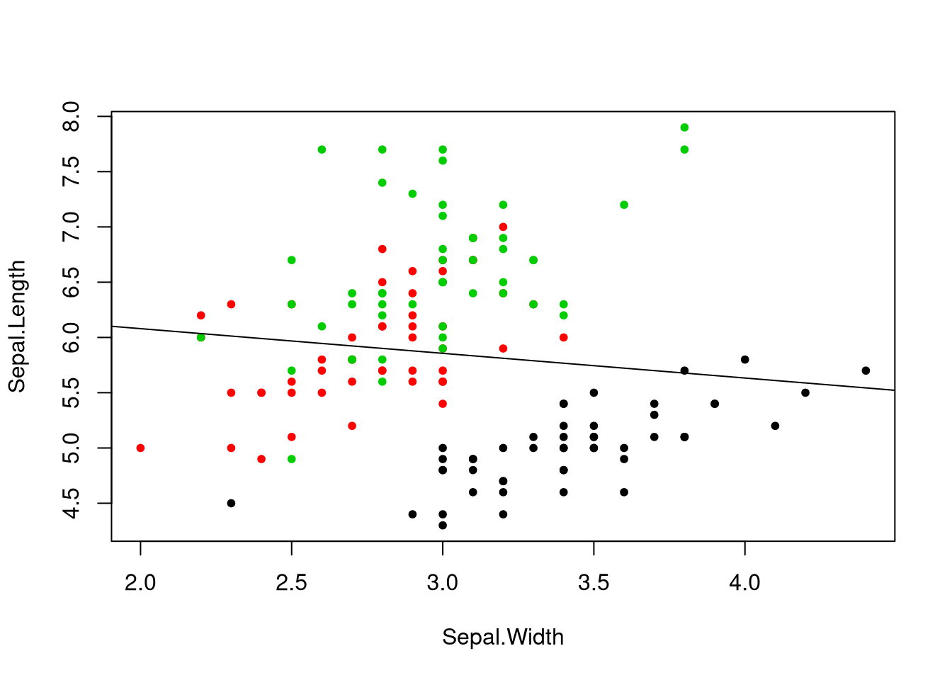
Do you notice something odd about this line? It’s a downward-sloping line, but
if we look at individual groups in the data, we see what appears to be a
positive relationship between sepal length and width. This is a phenomenon known
as Simpson’s paradox, where the trend line in subgroups differs with the
trend line across groups. In this case, setosa flower tend to have larger sepal
widths but lower length than the other flowers, yet there’s still a positive
relationship between the two. Perhaps instead we should disaggregate and look at
the regression line for only setosa flowers. Fortunately lm() provides an easy
interface for selecting a subset of a data set.
##
## Call:
## lm(formula = Sepal.Length ~ Sepal.Width, data = iris, subset = Species ==
##     "setosa")
##
## Coefficients:
## (Intercept)  Sepal.Width
##      2.6390       0.6905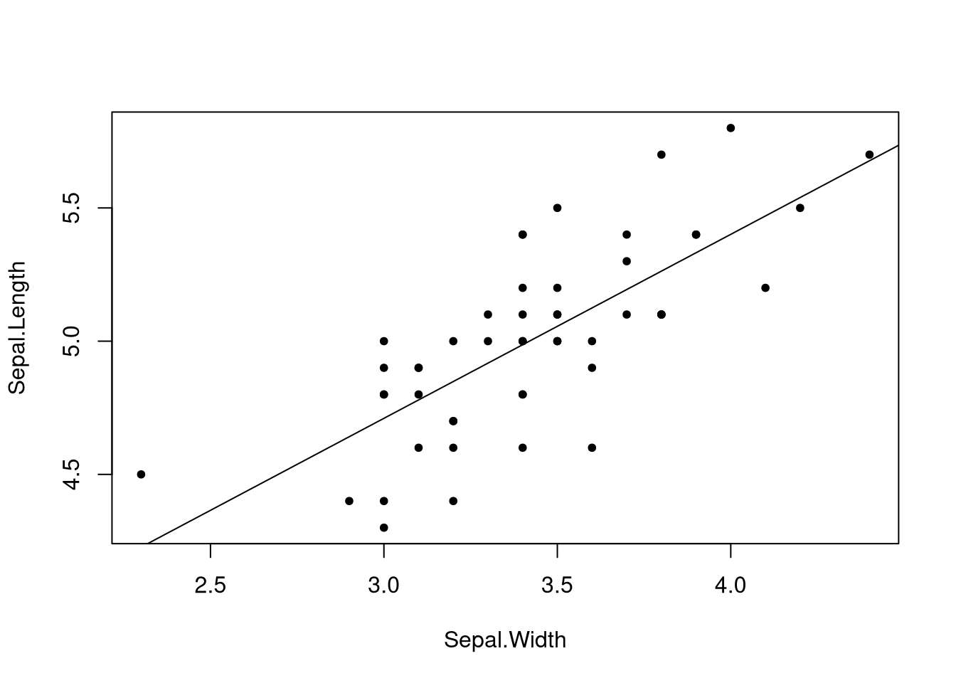
That line makes much more sense.
What if we want to call a function on our variables or apply some transformation to them? We can use function calls in formulas. For example, if we wanted to attempt to fit a log model to our data, we could do so like so:
##
## Call:
## lm(formula = log(Sepal.Length) ~ Sepal.Width, data = iris, subset = Species ==
##     "setosa")
##
## Coefficients:
## (Intercept)  Sepal.Width
## 1.1368 0.1375##
## Call:
## lm(formula = Sepal.Length ~ log(Sepal.Width), data = iris, subset = Species ==
## "setosa")
##
## Coefficients:
## (Intercept) log(Sepal.Width)
## 2.202 2.287However, for operations such as ^ or * that have special meaning in
formulas, you should call such operations using I(), like so:
##
## Call:
## lm(formula = Sepal.Length ~ I(Sepal.Width^2), data = iris, subset = Species ==
##     "setosa")
##
## Coefficients:
##      (Intercept)  I(Sepal.Width^2)
##           3.8113            0.1005
A handy function is the scale() function which centers the data around its
mean and subtracts out the standard deviation.
##        Sepal.Length
##   [1,]          5.1  1.01560199
##   [2,]          4.9 -0.13153881
##   [3,]          4.7  0.32731751
##   [4,]          4.6  0.09788935
##   [5,]          5.0  1.24503015
##   [6,]          5.4  1.93331463
##   [7,]          4.6  0.78617383
##   [8,]          5.0  0.78617383
##   [9,]          4.4 -0.36096697
##  [10,]          4.9  0.09788935
##  [11,]          5.4  1.47445831
##  [12,]          4.8  0.78617383
##  [13,]          4.8 -0.13153881
##  [14,]          4.3 -0.13153881
##  [15,]          5.8  2.16274279
##  [16,]          5.7  3.08045544
##  [17,]          5.4  1.93331463
##  [18,]          5.1  1.01560199
##  [19,]          5.7  1.70388647
##  [20,]          5.1  1.70388647
##  [21,]          5.4  0.78617383
##  [22,]          5.1  1.47445831
##  [23,]          4.6  1.24503015
##  [24,]          5.1  0.55674567
##  [25,]          4.8  0.78617383
##  [26,]          5.0 -0.13153881
##  [27,]          5.0  0.78617383
##  [28,]          5.2  1.01560199
##  [29,]          5.2  0.78617383
##  [30,]          4.7  0.32731751
##  [31,]          4.8  0.09788935
##  [32,]          5.4  0.78617383
##  [33,]          5.2  2.39217095
##  [34,]          5.5  2.62159911
##  [35,]          4.9  0.09788935
##  [36,]          5.0  0.32731751
##  [37,]          5.5  1.01560199
##  [38,]          4.9  1.24503015
##  [39,]          4.4 -0.13153881
##  [40,]          5.1  0.78617383
##  [41,]          5.0  1.01560199
##  [42,]          4.5 -1.73753594
##  [43,]          4.4  0.32731751
##  [44,]          5.0  1.01560199
##  [45,]          5.1  1.70388647
##  [46,]          4.8 -0.13153881
##  [47,]          5.1  1.70388647
##  [48,]          4.6  0.32731751
##  [49,]          5.3  1.47445831
##  [50,]          5.0  0.55674567
##  [51,]          7.0  0.32731751
##  [52,]          6.4  0.32731751
##  [53,]          6.9  0.09788935
##  [54,]          5.5 -1.73753594
##  [55,]          6.5 -0.59039513
##  [56,]          5.7 -0.59039513
##  [57,]          6.3  0.55674567
##  [58,]          4.9 -1.50810778
##  [59,]          6.6 -0.36096697
##  [60,]          5.2 -0.81982329
##  [61,]          5.0 -2.42582042
##  [62,]          5.9 -0.13153881
##  [63,]          6.0 -1.96696410
##  [64,]          6.1 -0.36096697
##  [65,]          5.6 -0.36096697
##  [66,]          6.7  0.09788935
##  [67,]          5.6 -0.13153881
##  [68,]          5.8 -0.81982329
##  [69,]          6.2 -1.96696410
##  [70,]          5.6 -1.27867961
##  [71,]          5.9  0.32731751
##  [72,]          6.1 -0.59039513
##  [73,]          6.3 -1.27867961
##  [74,]          6.1 -0.59039513
##  [75,]          6.4 -0.36096697
##  [76,]          6.6 -0.13153881
##  [77,]          6.8 -0.59039513
##  [78,]          6.7 -0.13153881
##  [79,]          6.0 -0.36096697
##  [80,]          5.7 -1.04925145
##  [81,]          5.5 -1.50810778
##  [82,]          5.5 -1.50810778
##  [83,]          5.8 -0.81982329
##  [84,]          6.0 -0.81982329
##  [85,]          5.4 -0.13153881
##  [86,]          6.0  0.78617383
##  [87,]          6.7  0.09788935
##  [88,]          6.3 -1.73753594
##  [89,]          5.6 -0.13153881
##  [90,]          5.5 -1.27867961
##  [91,]          5.5 -1.04925145
##  [92,]          6.1 -0.13153881
##  [93,]          5.8 -1.04925145
##  [94,]          5.0 -1.73753594
##  [95,]          5.6 -0.81982329
##  [96,]          5.7 -0.13153881
##  [97,]          5.7 -0.36096697
##  [98,]          6.2 -0.36096697
##  [99,]          5.1 -1.27867961
## [100,]          5.7 -0.59039513
## [101,]          6.3  0.55674567
## [102,]          5.8 -0.81982329
## [103,]          7.1 -0.13153881
## [104,]          6.3 -0.36096697
## [105,]          6.5 -0.13153881
## [106,]          7.6 -0.13153881
## [107,]          4.9 -1.27867961
## [108,]          7.3 -0.36096697
## [109,]          6.7 -1.27867961
## [110,]          7.2  1.24503015
## [111,]          6.5  0.32731751
## [112,]          6.4 -0.81982329
## [113,]          6.8 -0.13153881
## [114,]          5.7 -1.27867961
## [115,]          5.8 -0.59039513
## [116,]          6.4  0.32731751
## [117,]          6.5 -0.13153881
## [118,]          7.7  1.70388647
## [119,]          7.7 -1.04925145
## [120,]          6.0 -1.96696410
## [121,]          6.9  0.32731751
## [122,]          5.6 -0.59039513
## [123,]          7.7 -0.59039513
## [124,]          6.3 -0.81982329
## [125,]          6.7  0.55674567
## [126,]          7.2  0.32731751
## [127,]          6.2 -0.59039513
## [128,]          6.1 -0.13153881
## [129,]          6.4 -0.59039513
## [130,]          7.2 -0.13153881
## [131,]          7.4 -0.59039513
## [132,]          7.9  1.70388647
## [133,]          6.4 -0.59039513
## [134,]          6.3 -0.59039513
## [135,]          6.1 -1.04925145
## [136,]          7.7 -0.13153881
## [137,]          6.3  0.78617383
## [138,]          6.4  0.09788935
## [139,]          6.0 -0.13153881
## [140,]          6.9  0.09788935
## [141,]          6.7  0.09788935
## [142,]          6.9  0.09788935
## [143,]          5.8 -0.81982329
## [144,]          6.8  0.32731751
## [145,]          6.7  0.55674567
## [146,]          6.7 -0.13153881
## [147,]          6.3 -1.27867961
## [148,]          6.5 -0.13153881
## [149,]          6.2  0.78617383
## [150,] 5.9 -0.13153881##
## Call:
## lm(formula = scale(Sepal.Length) ~ scale(Sepal.Width), data = iris,
## subset = Species == "setosa")
##
## Coefficients:
## (Intercept) scale(Sepal.Width)
## -1.3203 0.3635Note that the interpretation of the coefficients when computed on scaled data differs from the interpretation for unscaled data.
Above a line was plotted. This line represents the predicted sepal lengths given
the sepal widths. It’s possible to get predicted values at specific points on
the line, for specific sepal widths. The function predict() (a generic
function) gets predicted values. To use it, one must give a data frame
resembling the one from which the model was estimated, except perhaps leaving
out the variable we’re attempting to predict.
##        1        2        3        4        5        6        7        8
## 5.055715 4.710470 4.848568 4.779519 5.124764 5.331911 4.986666 4.986666
##        9       10       11       12       13       14       15       16
## 4.641421 4.779519 5.193813 4.986666 4.710470 4.710470 5.400960 5.677156
##       17       18       19       20       21       22       23       24
## 5.331911 5.055715 5.262862 5.262862 4.986666 5.193813 5.124764 4.917617
##       25       26       27       28       29       30       31       32
## 4.986666 4.710470 4.986666 5.055715 4.986666 4.848568 4.779519 4.986666
##       33       34       35       36       37       38       39       40
## 5.470009 5.539058 4.779519 4.848568 5.055715 5.124764 4.710470 4.986666
##       41       42       43       44       45       46       47       48
## 5.055715 4.227128 4.848568 5.055715 5.262862 4.710470 5.262862 4.848568
##       49       50
## 5.193813 4.917617## 1 2 3
## 4.019981 4.710470 5.400960When making predictions, though, you should avoid extrapolation, which is making predictions outside of the range of the data. Going slightly outside the range of the data is fine, but well outside the range is a problem. We will talk later about estimating prediction errors, but leaving the range of the data tends to produce predictions with high error. More importantly, though, while a linear model may be appropriate in a certain range of the data, the same linear model may not be appropriate outside of the range; data might be locally linear rather than globally linear. This means that outside of the range the model is likely to be wrong, and a different model should be used. Since no data was observed in that range, though, determining and estimating that model is hard.