Lecture 9
Random Number Generation
Computers cannot create random numbers. They are Turing-complete, and a Turing machine is deterministic, not random. Instead, computers generate pseudo-random numbers. They start with a seed, an initial number in a sequence, and from there generate further numbers in the sequence that, without knowing the initial seed, appear to be random. That said, if the seed were known along with the generating process, the random sequence could be recreated exactly. Usually the system time is used to initialize a random number generator, since this may look random to a user. In R, you can use the set.seed() function to set a random seed. With no parameters, R will reset the random seed. If you wish to set the seed to a specific (numeric) value, you can do so with set.seed(seed). (You do not have to set a seed; R will automatically pick one at the start of a session, though if you want reproducible results, you should set the seed and communicate what it is.) For this document, I set the seed below.
set.seed(52716)Random number generators generate uniformly distributed random numbers. Once they can generate random numbers from the uniform distribution, random numbers following other distributions can be generated as well, so only one random number generator is needed.
The sample() function allows for some basic random value generation. Two arguments are required. The first is a vector containing the values that could be generated. This is your sample space, the possible values that could be generated by the random process. The second is the number of random values to generate. The call sample(x, size) will generate a random vector consisting of values from x of length size.
# Here I simulate the classic ball-in-bag probability model where random
# balls are pulled from a bag, without replacement. There are 32 red balls
# and 16 blue balls. I pull five balls from the bag.
sample(rep(c("red", "blue"), times = c(32, 16)), 5)
## [1] "blue" "red" "red" "red" "red"By default, sample() will use a model where random values are generated without replacement. This means that once a value is observed, it cannot be observed again (in the ball-and-bag model, this equates to pulling a ball from the bag and not putting the ball back in; once drawn, it cannot be drawn again). This naturally means that you must have size < length(x), or an error will be thrown; you can’t draw random values when you run out! To switch to a model with replacement (i.e. balls are put back in the bag after being drawn), set the parameter replace = TRUE.
# A model without replacement
ball_pull1 <- sample(rep(c("red", "blue"), times = c(32, 16)), 32 + 16)
ball_pull1
## [1] "red" "red" "red" "red" "blue" "blue" "blue" "blue" "red" "red"
## [11] "blue" "red" "red" "red" "red" "red" "blue" "blue" "red" "red"
## [21] "red" "red" "red" "blue" "red" "red" "red" "blue" "red" "red"
## [31] "blue" "red" "blue" "blue" "red" "red" "red" "blue" "red" "red"
## [41] "blue" "red" "red" "red" "red" "blue" "red" "blue"# Since I pulled all balls out of the bag, I get exactly 32 reds and 16
# blues
table(ball_pull1)## ball_pull1
## blue red
## 16 32# Now with replacement
ball_pull2 <- sample(rep(c("red", "blue"), times = c(32, 16)), 32 + 16, replace = TRUE)
ball_pull2## [1] "red" "red" "red" "blue" "red" "red" "red" "red" "blue" "red"
## [11] "red" "red" "red" "red" "red" "blue" "red" "red" "red" "red"
## [21] "red" "red" "red" "red" "red" "blue" "red" "red" "blue" "red"
## [31] "red" "red" "red" "red" "red" "red" "blue" "red" "red" "blue"
## [41] "red" "red" "blue" "red" "blue" "red" "red" "blue"# While close to the true frequencies, I don't see red balls exactly 32
# times, or blue balls exactly 16 times.
table(ball_pull2)## ball_pull2
## blue red
## 10 38By default, sample() will assume that each element in x is equally likely. This can be changed by setting prob to a vector assigning probabilities to each outcome.
# We can change the sampling with replacement model by making the sample
# space only c('red', 'blue'), and setting the probability of seeing these
# respective values to those consistent with our model.
sample(c("red", "blue"), 5, replace = TRUE, prob = c(32/48, 16/48))
## [1] "red" "red" "red" "red" "blue"Families of Distributions
R facilitates both description and simulation of random variables from various families of probability distributions, using similar formats. Each family will have four R functions associated with it, preceded by a character and followed by the identifier of the family.
dfunctions are associated with the probability density function (pdf) or probability mass function (pmf) of a distribution. An input vector of quantiles will get the value of the pdf/pmf at those quantiles.pfunctions are associated with the cumulative distribution function (cdf) of a probability distribution. Thus they describe the probability \(P(X \leq x)\), or the probability of being less than the input. This is often referred to as the lower tail of the distribution. If instead you want the upper tail, or \(P(X > x)\), you can setlower.tail = FALSEin apfunction to obtain the upper tail.qfunctions are associated with the quantiles of the probability distribution, and thus are the inverse of the cdf. There is likewise alower.tailparameter for theqfunction.rfunctions generate random values drawn from the distribution.
I give examples below for some distributions, starting with some discrete distributions.
Bernoulli
A Bernoulli random variable is a random variable that is either 1 or 0, and is described by the probability of obtaining 1, often denoted \(p\). Thus we denote a Bernoulli random variable with:
\[X \sim \operatorname{Ber}(p)\]
Note that if \(p = \frac{1}{2}\), this is the model of a single fair coin flip.
Bellow, I plot the pdf’s and cdf’s of a random variable \(X \sim \operatorname{Ber}(\frac{1}{2})\), and also simulate some values.
# I will be plotting a lot of pmf's in this document, so I create a function
# to help save effort.  The first argument, q, represents the quantiles of
# the random variable (the values that are possible). The second argument
# represents the value of the pmf at each q (and thus should be of the same
# length); in other words, for each q, p is the probability of seeing q
plot_pmf <- function(q, p) {
    # This will plot a series of horizontal lines at q with height p, setting
    # the y limits to a reasonable heights
    plot(q, p, type = "h", xlab = "x", ylab = "probability", main = "pmf", ylim = c(0,
        max(p) + 0.1))
    # Usually these plots have a dot at the end of the line; the point function
    # will add these dots to the plot created above
    points(q, p, pch = 16, cex = 2)
}

# Plot the pmf of a Bernoulli rv
ber_q <- c(0, 1)
ber_pmf <- dbinom(ber_q, 1, 0.5)
plot_pmf(ber_q, ber_pmf)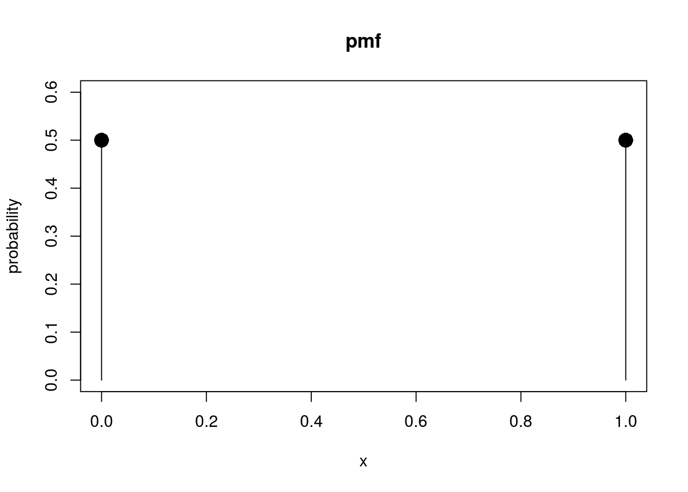
# Plot the cdf of a Bernoulli rv
ber_q2 <- seq(-1, 2, length = 1000)
ber_cdf <- pbinom(ber_q2, 1, 0.5)
# Plot the cdf with a line plot
plot(ber_q2, ber_cdf, type = "l", xlab = "x", ylab = "probability", main = "cdf",
    ylim = c(0, 1.1))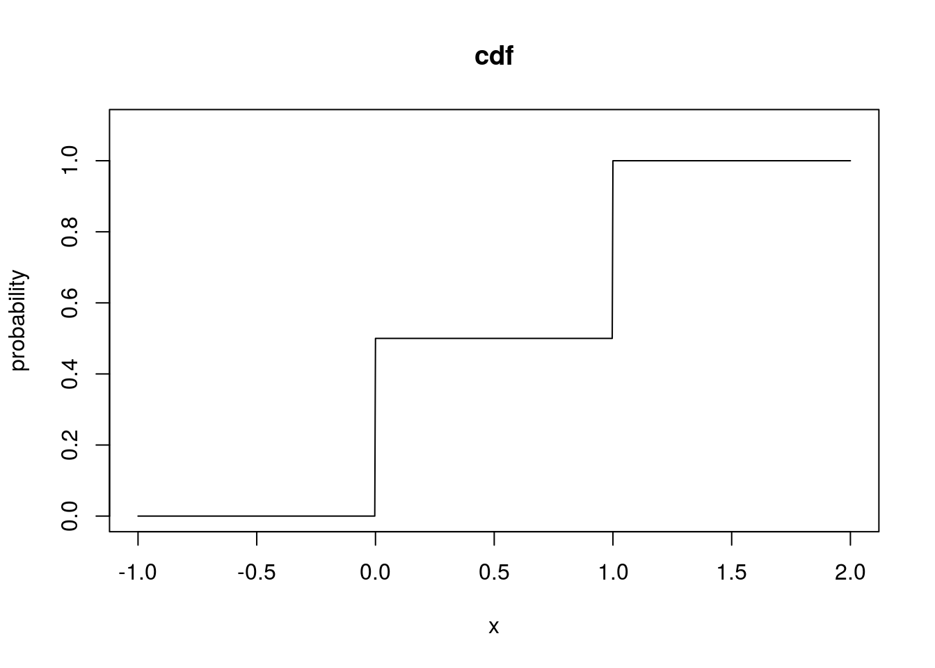
# The quartiles of a Bernoulli distribution
qbinom(seq(0, 1, by = 0.25), 1, 0.5)
## [1] 0 0 0 1 1# Generate 10 random values from a Bernoulli distribution
rbinom(10, 1, 0.5)## [1] 1 0 0 1 1 0 0 0 1 1Binomial
A binomial random variable is specified by two parameters, \(n\) and \(p\), and is denoted by:
\[X \sim \operatorname{BINOM}(n, p)\]
Binomial random variables represent the number of times \(n\) Bernoulli random variables are 1 when the probability of seeing 1 is \(p\) (another way to think of this is that if a coin flip is a Bernoulli random variable, then the number of times the coin lands heads-up when flipped \(n\) times is a binomial random variable).
The functions for the binomial distribution are dbinom(), pbinom(), qbinom(), and rbinom(). All of these have arguments size and prob for specifying the parameters n and p of the binomial distribution respectively.
# Let's consider a model where a fair coin is flipped five times.  The pmf
# of the binomial rv:
binom_q <- 0:5
binom_pmf <- dbinom(binom_q, size = 5, prob = 0.5)
plot_pmf(binom_q, binom_pmf)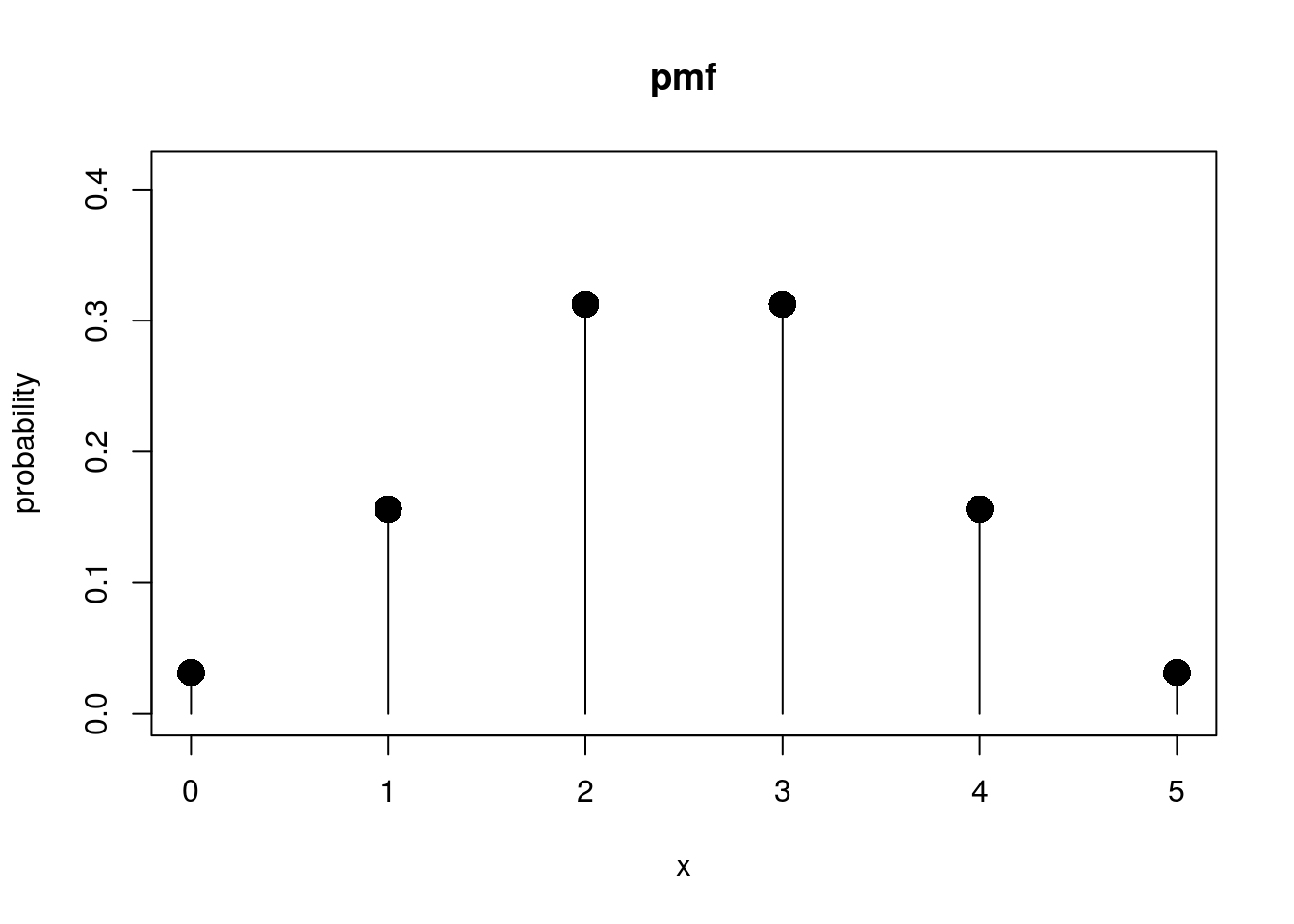
# The cdf of a binomial rv
binom_q2 <- seq(-1, 6, length = 1000)
binom_cdf <- pbinom(binom_q2, size = 5, prob = 0.5)
plot(binom_q2, binom_cdf, type = "l", xlab = "x", ylab = "probability", main = "cdf",
    ylim = c(0, 1.1))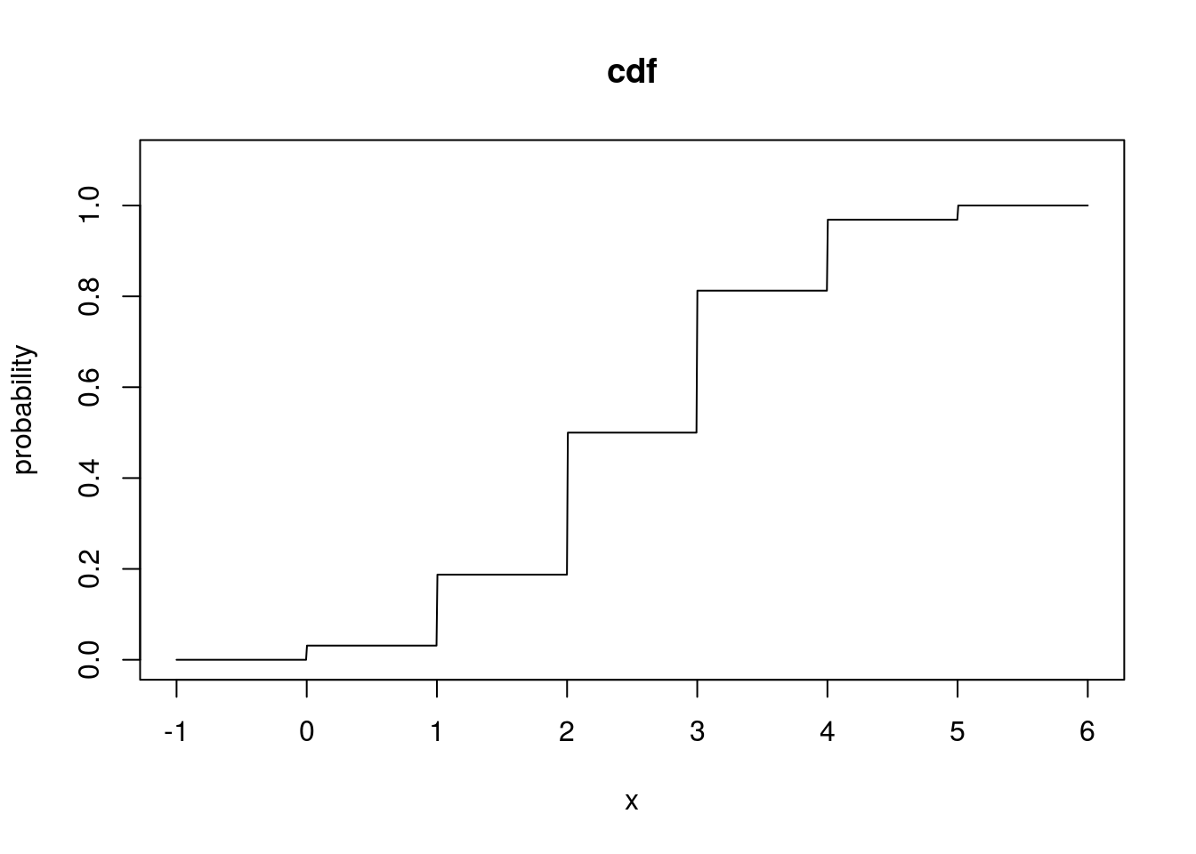
# The quartiles of this binomial rv
qbinom(seq(0, 1, by = 0.25), size = 5, prob = 0.5)
## [1] 0 2 2 3 5# 10 simulated binomial rv
rbinom(10, size = 5, prob = 0.5)## [1] 3 3 3 5 4 3 2 2 1 2Geometric
A geometric random variable is specified by one parameter, \(p\), and is denoted by:
\[X \sim \operatorname{GEOM}(p)\]
This random variable represents how many times a Bernoulli random variable with parameter \(p\) is created until a 1 is seen. (In other words, the number of times a coin is flipped until it lands heads-up is a geometric random variable). The name comes from the fact that the pmf of a geometric random variable is a geometric series, or \(p(x) = p(1 - p)^{x - 1}\).
The functions for working with geometric random variables are dgeom(), pgeom(), qgeom(), and rgeom(). All of these have an argument prob used to represent the parameter p of the geometric distribution.
# In these examples we will work with a geometric rv where p = 1. I now show
# part of its pmf
geom_q <- 0:20
geom_pmf <- dgeom(geom_q, prob = 0.1)
plot_pmf(geom_q, geom_pmf)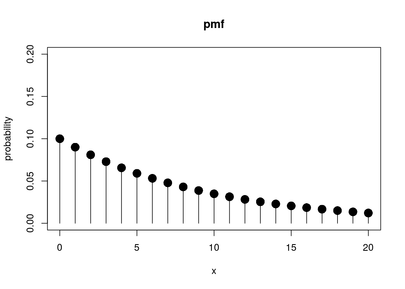
# The cdf of this variable
geom_q2 <- seq(-1, 21, length = 1000)
geom_cdf <- pgeom(geom_q2, prob = 0.1)
plot(geom_q2, geom_cdf, type = "l", xlab = "x", ylab = "probability", main = "cdf",
    ylim = c(0, 1.1))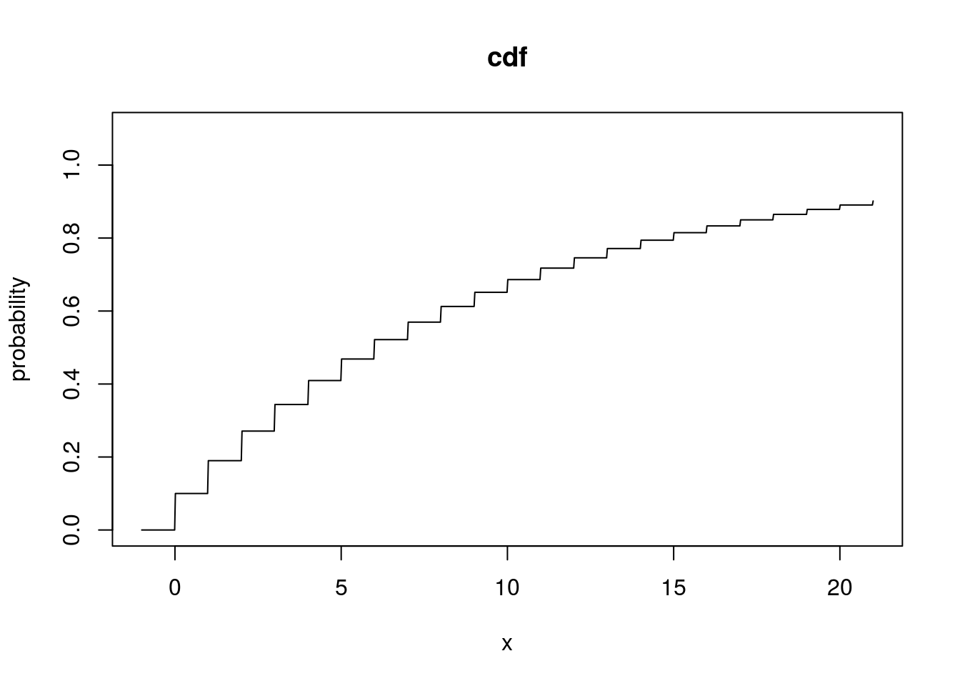
# Quartiles of a geometric rv
qgeom(seq(0, 1, by = 0.25), prob = 0.1)
## [1] 0 2 6 13 Inf# 10 simulated geometric rv's
rgeom(10, prob = 0.1)## [1] 19 3 11 8 10 4 14 13 11 0Poisson
A Poisson random variable is specified by one parameter, \(\lambda\), and is denoted by:
\[X \sim \operatorname{POI}(\lambda)\]
Poisson random variables are used to model counts of an event that occur in a finite frame of time. They are, in some sense, the inverse of a geometric random variable; while a geometric random variable represents the length of time to see one “success”, a Poisson random variable represents how many “successes” given a certain length of time. The parameter \(\lambda\) represents the average “success” rate. Some examples of Poisson random variables include:
- The number of calls a call center receives in a work day.
- How many goals a soccer team scores in a game.
- The number of deaths from horse kicks in the Prussian army annually.
The R functions for working with Poisson random variables are dpois(), ppois(), qpois(), and rpois(). The argument lambda corresponds to the parameter \(\lambda\).
# For these examples, the average success rate is 4.  Creating a pmf:
pois_q <- 0:20
pois_pmf <- dpois(pois_q, lambda = 4)
plot_pmf(pois_q, pois_pmf)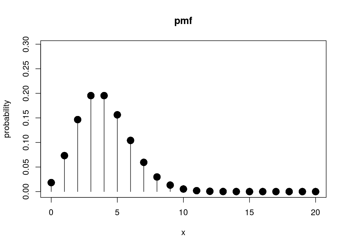
# Creating a cdf
pois_q2 <- seq(-1, 21, length = 1000)
pois_cdf <- ppois(pois_q2, lambda = 4)
plot(pois_q2, pois_cdf, type = "l", xlab = "x", ylab = "probability", main = "cdf",
    ylim = c(0, 1.1))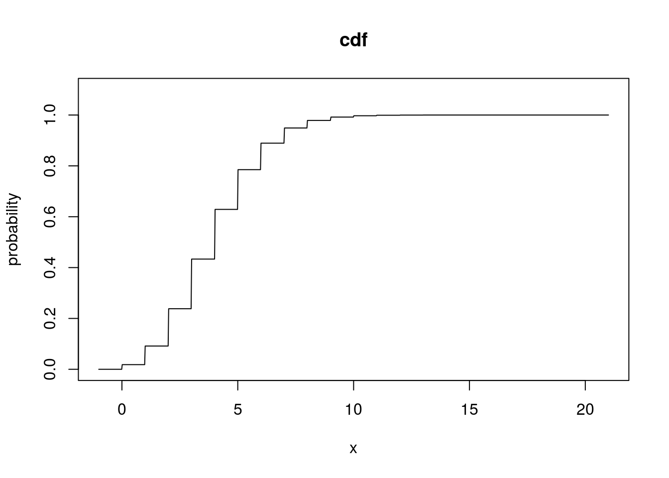
# Quartiles of the Poisson rv
qpois(seq(0, 1, by = 0.25), lambda = 4)
## [1] 0 3 4 5 Inf# Simulating Poisson rv's
rpois(10, lambda = 4)## [1] 4 5 2 4 4 5 3 3 2 0Uniform
The first continuous random variable I consider here is a uniformly distributed random variable, which is described by two parameters, \(a\) and \(b\), and represented with:
\[X \sim \operatorname{UNIF}(a, b)\]
\(a\) is the smallest value possible a uniformly distributed rv could take, and \(b\) the largest. Every number between \(a\) and \(b\) is equally weighted. It is a very important random variable, since it describes the probability for any random variable the probability that the random variable is a certain quantile of its distribution. Additionally, computers simulate uniform random variables, and using them you can simulate every other random variable.
The dunif(), punif(), qunif(), and runif() functions are used for working with uniform rv’s in R. They all have arguments min and max that correspond to parameters \(a\) and \(b\) mentioned above.
Being a continuous random variable, rather than having a pmf, a probability density function (pdf) is used for describing the random variable.
# Throughout I will set a = 0 and b = 1. This could be considered the
# standard Uniform random variable.  The pdf of a uniform rv:
unif_q <- seq(-1, 2, length = 1000)
unif_pdf <- dunif(unif_q, min = 0, max = 1)
plot(unif_q, unif_pdf, type = "l", xlab = "x", ylab = "density", main = "pdf",
    ylim = c(0, max(unif_pdf) + 0.1))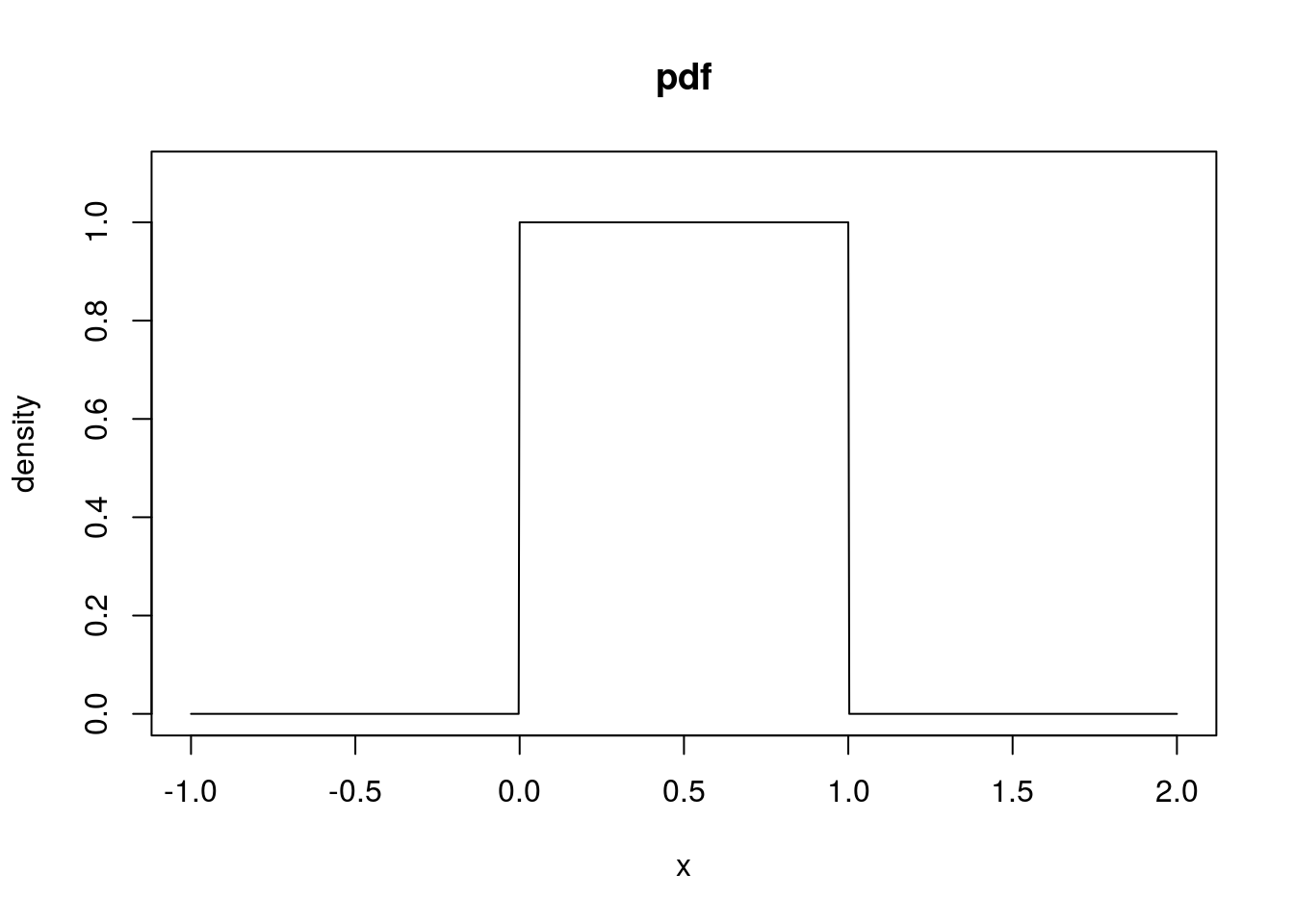
# The cdf of a uniform rv
unif_cdf <- punif(unif_q, min = 0, max = 1)
plot(unif_q, unif_cdf, type = "l", xlab = "x", ylab = "probability", main = "cdf",
    ylim = c(0, 1.1))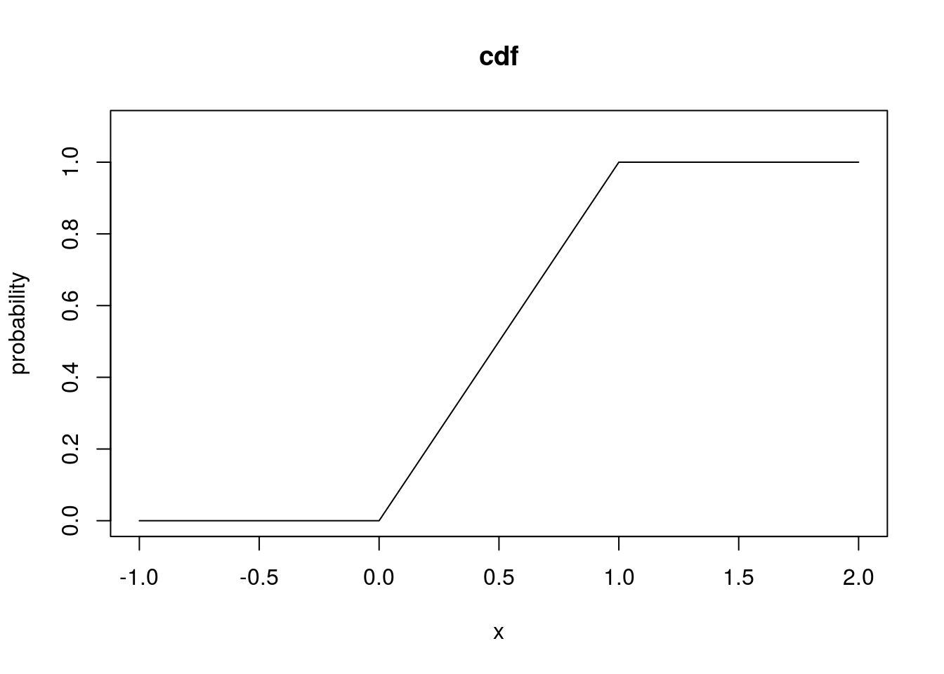
# Quartiles of a uniform rv
qunif(seq(0, 1, by = 0.25), min = 0, max = 1)
## [1] 0.00 0.25 0.50 0.75 1.00# Simulated uniform rv's
runif(10, min = 0, max = 1)## [1] 0.7562467 0.9696724 0.8479128 0.2943741 0.9111995 0.2399134 0.7144876
## [8] 0.3392606 0.8428848 0.8038884Exponential
The exponential distribution is specified by a parameter \(\mu\) and is described by:
\[X \sim \operatorname{EXP}(\mu)\]
\(\mu\) describes both the mean and the standard deviation of an exponential random variable. These are used to model waiting times, such as how long it takes a server to service a a customer and move on to the next one in the queue. Thus, \(\mu\) is the average length of time to service one customer and move on to the next. One could also consider instead \(\frac{1}{\mu}\), which is the rate at which customers are serviced. So if a call center takes on average half a minute to service a customer, the average rate at which it services its customers is two customers per minute. (You may notice some similarity between an exponential random variable and a geometric random variabe; the exponential rv is the continuous version of the geometric rv.)
The function dexp(), pexp(), qexp(), and rexp() are used for working with exponential random variables in R. You do not directly specify the mean wait time, \(\mu\), in R; instead you specify the rate, \(\frac{1}{\mu}\), with the rate argument. Thus if you wanted a mean of \(\mu = 6\), you would set rate = 1/6.
# Here we will model an exponential rv where the mean is 6. This means that
# the rate is 1/6.  The pdf of an exponential rv:
exp_q <- seq(-1, 12, length = 1000)
exp_pdf <- dexp(exp_q, rate = 1/6)
plot(exp_q, exp_pdf, type = "l", xlab = "x", ylab = "density", main = "pdf",
    ylim = c(0, max(exp_pdf) + 0.1))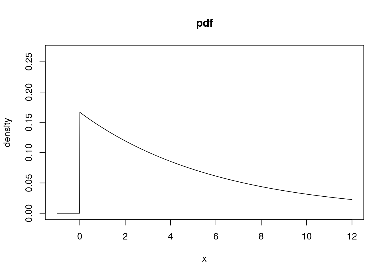
# The cdf of an exponential rv
exp_cdf <- pexp(exp_q, rate = 1/6)
plot(exp_q, exp_cdf, type = "l", xlab = "x", ylab = "probability", main = "cdf",
    ylim = c(0, 1.1))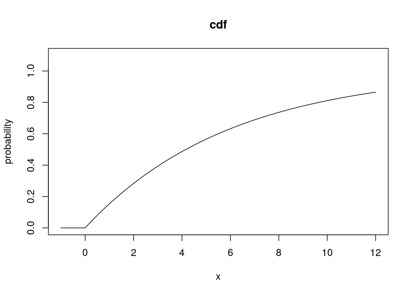
# Quartiles of an exponential rv
qexp(seq(0, 1, by = 0.25), rate = 1/6)
## [1] 0.000000 1.726092 4.158883 8.317766 Inf# Simulated exponential rv's
rexp(10, rate = 1/6)## [1] 4.181027 1.381246 2.254482 2.814817 1.777893 15.998047 13.546735
## [8] 13.562386 4.017361 4.070043Normal
The Normal distribution is specified by two parameter, \(\mu\) and \(\sigma\), and is described by:
\[X \sim N(\mu, \sigma)\]
\(\mu\) is the mean of a Normal rv, and \(\sigma\) is the rv’s standard deviation. The Normal distribution describes the distribution of “errors”, or now far away some random variable is from its mean. It is perhaps the most important distribution in probability and statistics.
The functions dnorm(), pnorm(), qnorm(), and rnorm() are used for working with Normal rv’s. They have two arguments, mean and sd, used for specifying the parameters \(\mu\) and \(\sigma\), respectively.
# We will set the mean to 10 and the standard deviation to 2 when working
# with Normal rv's in this example.  The pdf of a Normal rv:
norm_q <- seq(4, 16, length = 1000)
norm_pdf <- dnorm(norm_q, mean = 10, sd = 2)
plot(norm_q, norm_pdf, type = "l", xlab = "x", ylab = "density", main = "pdf",
    ylim = c(0, max(norm_pdf) + 0.1))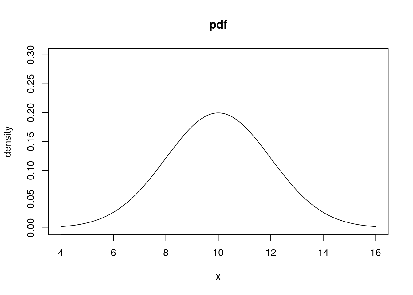
# The cdf of a Normal rv:
norm_cdf <- pnorm(norm_q, mean = 10, sd = 2)
plot(norm_q, norm_cdf, type = "l", xlab = "x", ylab = "probability", main = "cdf",
    ylim = c(0, 1.1))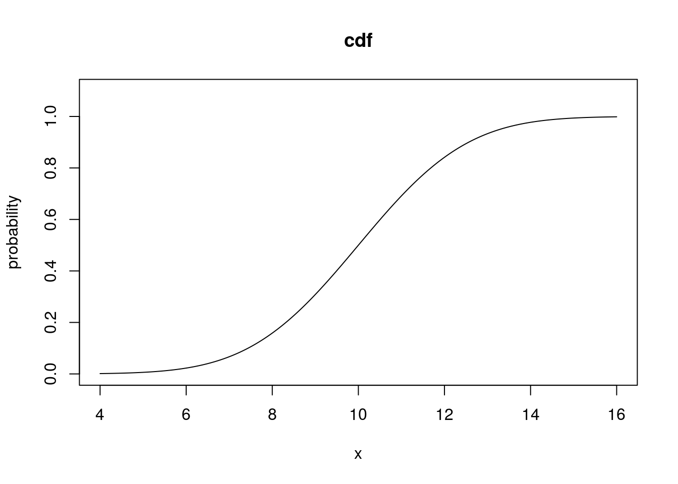
# The quartiles of a Normal rv
qnorm(seq(0, 1, by = 0.25), mean = 10, sd = 2)
## [1] -Inf 8.65102 10.00000 11.34898 Inf# Simulated Normal rv's
rnorm(10, mean = 10, sd = 2)## [1] 12.541297 11.221620 7.411588 13.483226 12.046666 8.065685 10.076769
## [8] 10.338442 7.755875 6.666931Central Limit Theorem
One of the most important theorems in all of statistics is the central limit theorem. This theorem describes the distribution of the sample mean as the sample size grows large. Let \(X_i\) be a random variable with mean \(\mu\) and standard deviation \(\sigma\). For every \(i\) such that \(1 \leq i \leq n\) (\(n\) representing the sample size), \(X_i\) is independent and identically distributed, or iid (meaning that every data point is drawn from the exact same distribution and do not depend on the value of other \(X_i\) in the data set). Let \(\overline{X} = \frac{1}{n}\sum_{i = 1}^{n} X_i\) be the sample mean of this data set. Then:
\[\overline{X} \sim N\left(\mu, \frac{\sigma}{\sqrt{n}}\right) \text{ as } n \to \infty\]
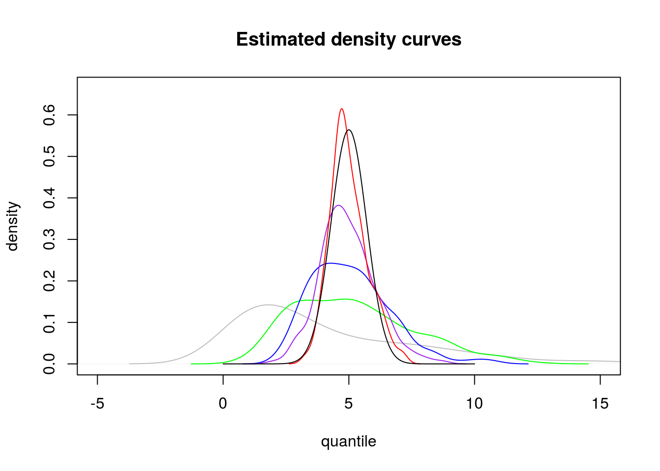
This is saying that if the above conditions hold, the distribution of the sample mean \(\overline{X}\) begins to resemble the Normal distribution with larger sample sizes, regardless of the original distribution of \(X_i\). This is the basis of much of statistical inference.
We can show the central limit theorem at work in R. Let \(X_i \sim \operatorname{EXP}(5)\). Notice that \(\mu = 5\) and \(\sigma = \mu = 5\). If the sample size is \(n\), the central limit theorem says that the distribution of \(\overline{X}\) should begin to resemble the Normal distribution with mean \(\mu = 5\) and standard deviation:
\[\frac{\sigma}{\sqrt{n}} = \frac{5}{\sqrt{n}}\]
as \(n\) grows large.
Let’s consider samples of size 10, 50, 200, and 1000. I first generate 200 simulated means from samples for each of these sizes.
# We will loop over the vector c(10, 50, 200, 500), each of these
# representing a sample size. lapply() applies a function (the second
# argument) to each element of this vector, and stores the result as a list,
# which we will call sim_means. The (anonymous) function will take only one
# argument, n, representing the sample size. It will return a vector of
# simulated means when the sample size is n.
sim_means <- lapply(c(5, 10, 20, 50), function(n) {
    # I now simulate 200 data sets of size n from the exponential distribution,
    # setting rate = 1/5 for exponentially distributed random variables with
    # mean 5, and store the resulting data sets in a list called sim_data_sets.
    # (I add a throwaway argument because something will be passed to the
    # function, but I don't want to use it)
    sim_data_sets <- lapply(1:200, function(throwaway) rexp(n, rate = 1/5))
    # Return a vector containing means for each of these data sets.
    sapply(sim_data_sets, mean)
})
# Let's look at what we just made
str(sim_means)
## List of 4
## $ : num [1:200] 3.51 4.13 2.59 2.91 4.67 ...
## $ : num [1:200] 5.38 3.29 5.43 2.68 4.21 ...
## $ : num [1:200] 4.01 2.83 6.64 6.62 7.09 ...
## $ : num [1:200] 7.06 5.27 5.61 4.31 4.78 ...# First, I plot an estimated density function for simulated exponential
# random variables with mean 5 (rate 1/5)
plot(density(rexp(200, rate = 1/5)), xlab = "quantile", ylab = "density", main = "Estimated density curves",
col = "gray", type = "l", xlim = c(-5, 15), ylim = c(0, dnorm(5, mean = 5,
sd = 5/sqrt(50)) + 0.1))
# I add density curves for each of the simulated means
lines(density(sim_means[[1]]), col = "green")
lines(density(sim_means[[2]]), col = "blue")
lines(density(sim_means[[3]]), col = "purple")
lines(density(sim_means[[4]]), col = "red")
# Finally, add a Normal curve showing what the distribution of the final
# sample mean should be near according to the central limit theorem
clt_norm_q <- seq(0, 10, length = 1000)
lines(clt_norm_q, dnorm(clt_norm_q, mean = 5, sd = 5/sqrt(50)), col = "black")