Lecture 7
Distribution Comparison
A common problem is determining whether two distributions of two samples are the same. While statistical tests can help answer this question, visualization techniques are also quite effective. Many of the plots we have seen can be adapted to compare distributions from independent samples.
One way to do so is to create two stem-and-leaf plots back-to-back, sharing common stems but having leaves from different data sets extending out in different directions. Base R will not do this, but the stem.leaf.backback() function in the aplpack package can create such a chart. stem.leaf.backback(x, y) will plot the distributions of the data in vectors x and y with a back-to-back stem-and-leaf plot. Here we use this function to examine the distribution of tooth lengths of guinea pigs given different supplements, contained in the ToothGrowth data set.
library(aplpack)## Loading required package: tcltkstr(ToothGrowth)## 'data.frame': 60 obs. of 3 variables:
## $ len : num 4.2 11.5 7.3 5.8 6.4 10 11.2 11.2 5.2 7 ...
## $ supp: Factor w/ 2 levels "OJ","VC": 2 2 2 2 2 2 2 2 2 2 ...
## $ dose: num 0.5 0.5 0.5 0.5 0.5 0.5 0.5 0.5 0.5 0.5 ...# The split function can split data vectors depending on a factor. Here,
# split will split len in ToothGrowth depending on the factor variable supp,
# creating a list with the two variables we want
len_split <- with(ToothGrowth, split(len, supp))
OJ <- len_split$OJ
VC <- len_split$VC
stem.leaf.backback(OJ, VC, rule.line = "Sturges")## ______________________________________
## 1 | 2: represents 12, leaf unit: 1
## OJ VC
## ______________________________________
## | 0* |4 1
## 4 9998| 0. |55677 6
## 7 440| 1* |011134 12
## 11 9765| 1. |55667788 (8)
## (9) 443332110| 2* |1233 10
## 10 977666555| 2. |5669 6
## 1 0| 3* |23 2
## | 3. |
## | 4* |
## ______________________________________
## n: 30 30
## ______________________________________We have seen comparative boxplots before; again, they can be quite useful for comparing distributions. Calling boxplot(x, y) with two data vectors x and y will compare the distributions of the data in the vectors x and y with a comparative boxplot.
boxplot(OJ, VC)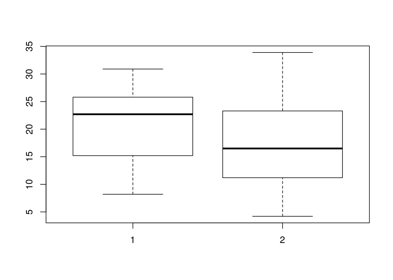
We can also use density estimates to compare distributions, like so:
plot(density(OJ), lty = 1)
lines(density(VC), lty = 2)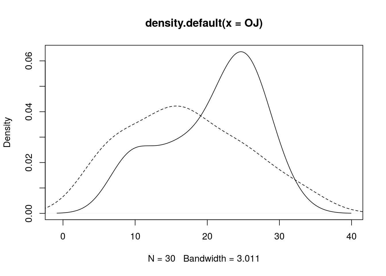
Model Formula Interface
You have seen this interface before, and now we discuss it in more detail. The interface is y ~ x, or more descriptively, response ~ predictor. Loosely, we see the response variable as being dependent on the predictor, which could by a single variable, as in y ~ x, or a combination of variables, as in y ~ x + z. (+ is overloaded to have a special meaning in the model formula interface, and thus does not necessarily mean “addition”. If you wish to have + mean literal “addition”, use the function I(), as in y ~ I(x + z).) Many function in R use the formula interface, and often include additional arguments such as data (for specifying a data frame containing the data and variables described by the formula) and subset (used for selecting a subset of the data, according to some logical rule). Functions that use this formula interface include boxplot(), lm(), summary(), and lattice plotting functions.
Below I demonstrate using boxplot()’s formula interface for exploring the ToothGrowth data more simply.
# Here, I plot the tooth growth data depending on supplement when dose ==
# 0.5
boxplot(len ~ supp, data = ToothGrowth, subset = dose == 0.5)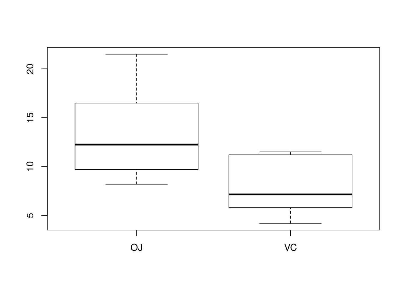
# I can create a boxplot that depends on both supplement and dosage
boxplot(len ~ supp + dose, data = ToothGrowth)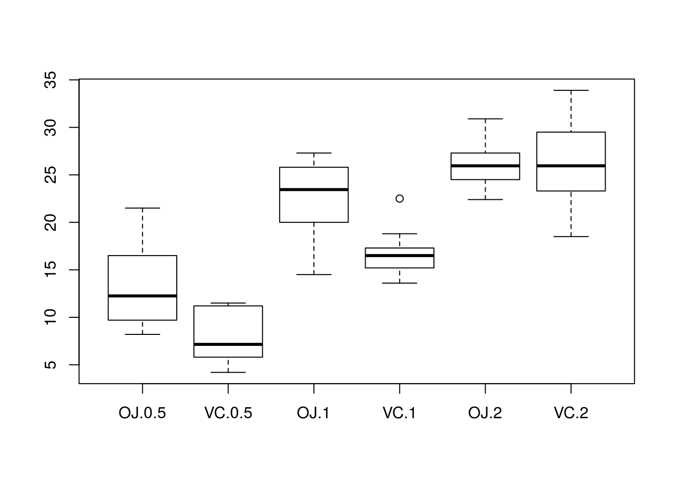
Here I compare means of tooth lengths using the formula interface in summary(), provided in the package Hmisc.
library(Hmisc)## Loading required package: lattice## Loading required package: survival## Loading required package: Formula## Loading required package: ggplot2##
## Attaching package: 'Hmisc'## The following objects are masked from 'package:base':
##
## format.pval, units# First, the result of summary
summary(len ~ supp + dose, data = ToothGrowth)## len N= 60
##
## +-------+---+--+--------+
## | | |N |len |
## +-------+---+--+--------+
## |supp |OJ |30|20.66333|
## | |VC |30|16.96333|
## +-------+---+--+--------+
## |dose |0.5|20|10.60500|
## | |1 |20|19.73500|
## | |2 |20|26.10000|
## +-------+---+--+--------+
## |Overall| |60|18.81333|
## +-------+---+--+--------+# A nice plot of this information (though the table is very informative; a
# plot may not be necessary)
plot(summary(len ~ supp + dose, data = ToothGrowth))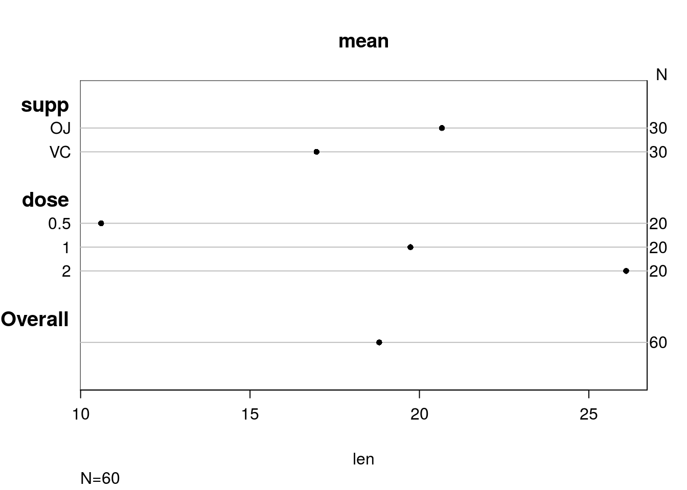
Splitting and Stacking Data
Consider the function boxplot(). We have seen two ways to make a parallel boxplot using boxplot(). One way is to have your data stored in separate vectors, say x and y, then call boxplot(x, y). Another way is to have the data stored in a data frame, say d, that has two columns, say v and g. The variable v contains the data stored in the original vectors x and y, and the variable g identifies whether the data belongs to group x or group y. Then the function call boxplot(v ~ g, data = d) will produce the same graphic we described earlier.
Which is the better approach? Here, there may not appear to be much difference. However, in other circumstances, it may be easier to have data stored in separate vectors or in a list containing those vectors (say, if you are using sapply() for looping), or it may be easier to have your data stored in “long form”, where a data frame contains the actual data points in one column and another column identifies the group to which each data point belongs (for example, if you are plotting using ggplot()). Thus it’s important to be able to transform data so it fits whichever format we need.
There are two functions that allow for an easy transition between these two formats: split() and stack(). split(v, g) will create a list of vectors where each data point in v is included in a vector identified by the vector g. (Naturally, v and g must be the same length.) For example, if tweet is a vector of strings representing tweets by Twitter users, and user is a vector that identifies the user who wrote each tweet stored in tweet, then l <- split(tweet, user) will create a list l with vectors for each unique user in user, each vector in the list containing the respective user’s tweets. So if NTGuardian is one of the users, l$NTGuardian is the vector containing NTGuardian’s tweets.
Let’s try this out on the iris data, where the Sepal.Length variable identifies sepal lengths of iris flowers, and Species identifies the species of each flower in the sample. Currently the data is in long form, so let’s separate it into separate vectors.
# A look at the data
head(iris)
## Sepal.Length Sepal.Width Petal.Length Petal.Width Species
## 1 5.1 3.5 1.4 0.2 setosa
## 2 4.9 3.0 1.4 0.2 setosa
## 3 4.7 3.2 1.3 0.2 setosa
## 4 4.6 3.1 1.5 0.2 setosa
## 5 5.0 3.6 1.4 0.2 setosa
## 6 5.4 3.9 1.7 0.4 setosa# It's in long form; let's change that
l <- split(iris$Sepal.Length, iris$Species)
l## $setosa
## [1] 5.1 4.9 4.7 4.6 5.0 5.4 4.6 5.0 4.4 4.9 5.4 4.8 4.8 4.3 5.8 5.7 5.4
## [18] 5.1 5.7 5.1 5.4 5.1 4.6 5.1 4.8 5.0 5.0 5.2 5.2 4.7 4.8 5.4 5.2 5.5
## [35] 4.9 5.0 5.5 4.9 4.4 5.1 5.0 4.5 4.4 5.0 5.1 4.8 5.1 4.6 5.3 5.0
##
## $versicolor
## [1] 7.0 6.4 6.9 5.5 6.5 5.7 6.3 4.9 6.6 5.2 5.0 5.9 6.0 6.1 5.6 6.7 5.6
## [18] 5.8 6.2 5.6 5.9 6.1 6.3 6.1 6.4 6.6 6.8 6.7 6.0 5.7 5.5 5.5 5.8 6.0
## [35] 5.4 6.0 6.7 6.3 5.6 5.5 5.5 6.1 5.8 5.0 5.6 5.7 5.7 6.2 5.1 5.7
##
## $virginica
## [1] 6.3 5.8 7.1 6.3 6.5 7.6 4.9 7.3 6.7 7.2 6.5 6.4 6.8 5.7 5.8 6.4 6.5
## [18] 7.7 7.7 6.0 6.9 5.6 7.7 6.3 6.7 7.2 6.2 6.1 6.4 7.2 7.4 7.9 6.4 6.3
## [35] 6.1 7.7 6.3 6.4 6.0 6.9 6.7 6.9 5.8 6.8 6.7 6.7 6.3 6.5 6.2 5.9# l can be used in sapply; say, we want the median sepal length for each
# flower
sapply(l, median)## setosa versicolor virginica
## 5.0 5.9 6.5# If we want the variables in the working environment, we will need to
# assign them to vectors manually
setosa <- l$setosa
versicolor <- l$versicolor
virginica <- l$virginica
# Make a density plot comparing the distributions
plot(density(virginica), lty = 1, ylim = c(0, 1.5))
lines(density(versicolor), lty = 2)
lines(density(setosa), lty = 3)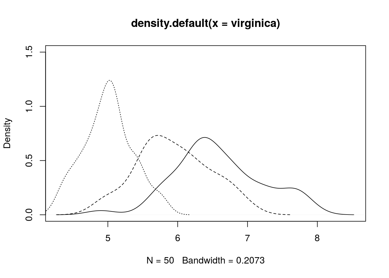
# This task lends naturally to the formula interface, and the DescTools
# package provides this interface
library(DescTools)
##
## Attaching package: 'DescTools'## The following objects are masked from 'package:Hmisc':
##
## Label, Mean, %nin%, Quantile## The following object is masked from 'package:aplpack':
##
## plot.bagplot# Notice this produces the same result as the earlier call
l2 <- split(Sepal.Length ~ Species, data = iris)
l2## $setosa
## [1] 5.1 4.9 4.7 4.6 5.0 5.4 4.6 5.0 4.4 4.9 5.4 4.8 4.8 4.3 5.8 5.7 5.4
## [18] 5.1 5.7 5.1 5.4 5.1 4.6 5.1 4.8 5.0 5.0 5.2 5.2 4.7 4.8 5.4 5.2 5.5
## [35] 4.9 5.0 5.5 4.9 4.4 5.1 5.0 4.5 4.4 5.0 5.1 4.8 5.1 4.6 5.3 5.0
##
## $versicolor
## [1] 7.0 6.4 6.9 5.5 6.5 5.7 6.3 4.9 6.6 5.2 5.0 5.9 6.0 6.1 5.6 6.7 5.6
## [18] 5.8 6.2 5.6 5.9 6.1 6.3 6.1 6.4 6.6 6.8 6.7 6.0 5.7 5.5 5.5 5.8 6.0
## [35] 5.4 6.0 6.7 6.3 5.6 5.5 5.5 6.1 5.8 5.0 5.6 5.7 5.7 6.2 5.1 5.7
##
## $virginica
## [1] 6.3 5.8 7.1 6.3 6.5 7.6 4.9 7.3 6.7 7.2 6.5 6.4 6.8 5.7 5.8 6.4 6.5
## [18] 7.7 7.7 6.0 6.9 5.6 7.7 6.3 6.7 7.2 6.2 6.1 6.4 7.2 7.4 7.9 6.4 6.3
## [35] 6.1 7.7 6.3 6.4 6.0 6.9 6.7 6.9 5.8 6.8 6.7 6.7 6.3 6.5 6.2 5.9stack() does the opposite of split(). stack() takes a list of vectors, named according to the group to which they belong, and returns a data frame with a column for the data and a column identifying the group to which each data point belongs. So if l is a list produced by split, stack(l) will return the data into the original long form format. Another example: if ff is a vector that contains the weight of boxes of Frosted Flakes cereals, trx a vector that contains the weights of boxes of Trix cereal, and ccp a vector that contains weights of boxes of Cocoa Puffs, then df <- stack(list("ff" = ff, "trx" = trx, "ccp" = ccp)) will create a data frame with a column containing weights of cereal boxes and a column containing the type of cereal.
Usage of stack() is demonstrated below.
# Recall setosa, versicolor, and verginica from before; let's reconstruct
# the data frame with which we made them.
setosa
## [1] 5.1 4.9 4.7 4.6 5.0 5.4 4.6 5.0 4.4 4.9 5.4 4.8 4.8 4.3 5.8 5.7 5.4
## [18] 5.1 5.7 5.1 5.4 5.1 4.6 5.1 4.8 5.0 5.0 5.2 5.2 4.7 4.8 5.4 5.2 5.5
## [35] 4.9 5.0 5.5 4.9 4.4 5.1 5.0 4.5 4.4 5.0 5.1 4.8 5.1 4.6 5.3 5.0versicolor## [1] 7.0 6.4 6.9 5.5 6.5 5.7 6.3 4.9 6.6 5.2 5.0 5.9 6.0 6.1 5.6 6.7 5.6
## [18] 5.8 6.2 5.6 5.9 6.1 6.3 6.1 6.4 6.6 6.8 6.7 6.0 5.7 5.5 5.5 5.8 6.0
## [35] 5.4 6.0 6.7 6.3 5.6 5.5 5.5 6.1 5.8 5.0 5.6 5.7 5.7 6.2 5.1 5.7virginica## [1] 6.3 5.8 7.1 6.3 6.5 7.6 4.9 7.3 6.7 7.2 6.5 6.4 6.8 5.7 5.8 6.4 6.5
## [18] 7.7 7.7 6.0 6.9 5.6 7.7 6.3 6.7 7.2 6.2 6.1 6.4 7.2 7.4 7.9 6.4 6.3
## [35] 6.1 7.7 6.3 6.4 6.0 6.9 6.7 6.9 5.8 6.8 6.7 6.7 6.3 6.5 6.2 5.9df <- stack(list(setosa = setosa, versicolor = versicolor, virginica = virginica))
head(df)## values ind
## 1 5.1 setosa
## 2 4.9 setosa
## 3 4.7 setosa
## 4 4.6 setosa
## 5 5.0 setosa
## 6 5.4 setosa# This is the ideal format for ggplot
library(ggplot2)
ggplot(df, aes(x = ind, y = values)) + geom_boxplot()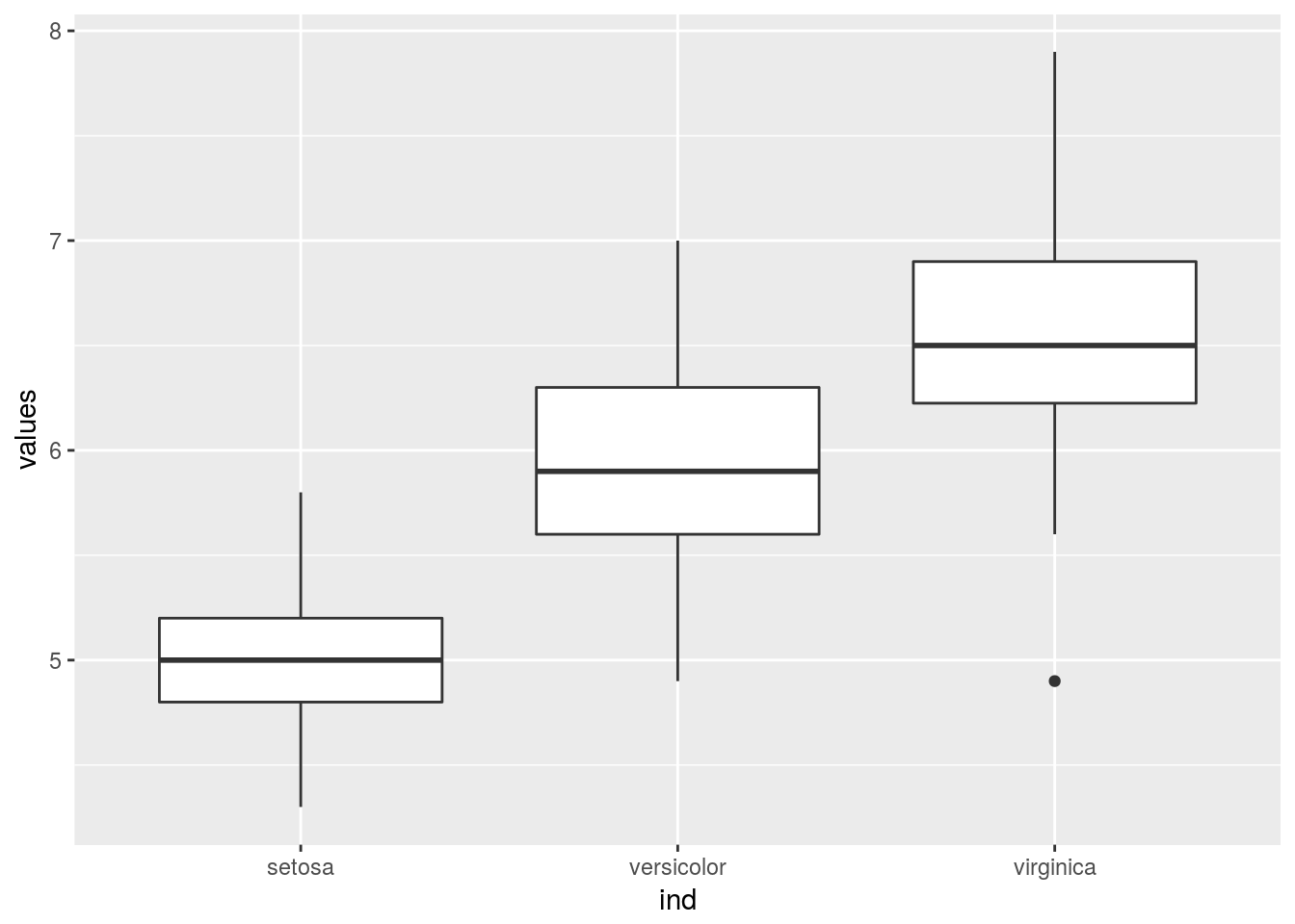
# To see that stack basically undoes what was done by split
head(ToothGrowth)
## len supp dose
## 1 4.2 VC 0.5
## 2 11.5 VC 0.5
## 3 7.3 VC 0.5
## 4 5.8 VC 0.5
## 5 6.4 VC 0.5
## 6 10.0 VC 0.5l <- with(ToothGrowth, split(len, supp))
l## $OJ
## [1] 15.2 21.5 17.6 9.7 14.5 10.0 8.2 9.4 16.5 9.7 19.7 23.3 23.6 26.4
## [15] 20.0 25.2 25.8 21.2 14.5 27.3 25.5 26.4 22.4 24.5 24.8 30.9 26.4 27.3
## [29] 29.4 23.0
##
## $VC
## [1] 4.2 11.5 7.3 5.8 6.4 10.0 11.2 11.2 5.2 7.0 16.5 16.5 15.2 17.3
## [15] 22.5 17.3 13.6 14.5 18.8 15.5 23.6 18.5 33.9 25.5 26.4 32.5 26.7 21.5
## [29] 23.3 29.5df2 <- stack(l)
head(df2)## values ind
## 1 15.2 OJ
## 2 21.5 OJ
## 3 17.6 OJ
## 4 9.7 OJ
## 5 14.5 OJ
## 6 10.0 OJ